Ch.30: Logistic Regression's Hyperparameters

Inspired by: YouTube

This closes out the Logistic Regression arc that started at Ch.20: the math, the loss function, gradient descent, softmax, polynomial features. scikit-learn's LogisticRegression exposes around 15 constructor parameters, and almost every one of them maps directly back to something already covered in this series. This post is a practical tour, grouped by what each knob actually controls.

1. Regularization: penalty, C, l1_ratio

penalty selects which regularization type gets added to the log loss: 'l1', 'l2', 'elasticnet', or None. These are exactly Lasso, Ridge, and Elastic Net's penalties (Ch.13 through Ch.19), applied to log loss instead of squared error. The default is 'l2'.

C controls how strong that regularization is, but with an inverted convention worth flagging explicitly: unlike Ridge/Lasso's alpha, where a bigger value means stronger regularization, C is defined as $\frac{1}{\lambda}$, so a smaller C means stronger regularization, and a larger C means weaker regularization (closer to plain, unregularized Logistic Regression). Default is 1.0.

l1_ratio only does anything when penalty='elasticnet', it's the same 0 to 1 mixing ratio between L1 and L2 from Ch.19, 0 behaves like pure Ridge, 1 like pure Lasso.

Seeing C's effect directly, fitting the same dataset at three different values:

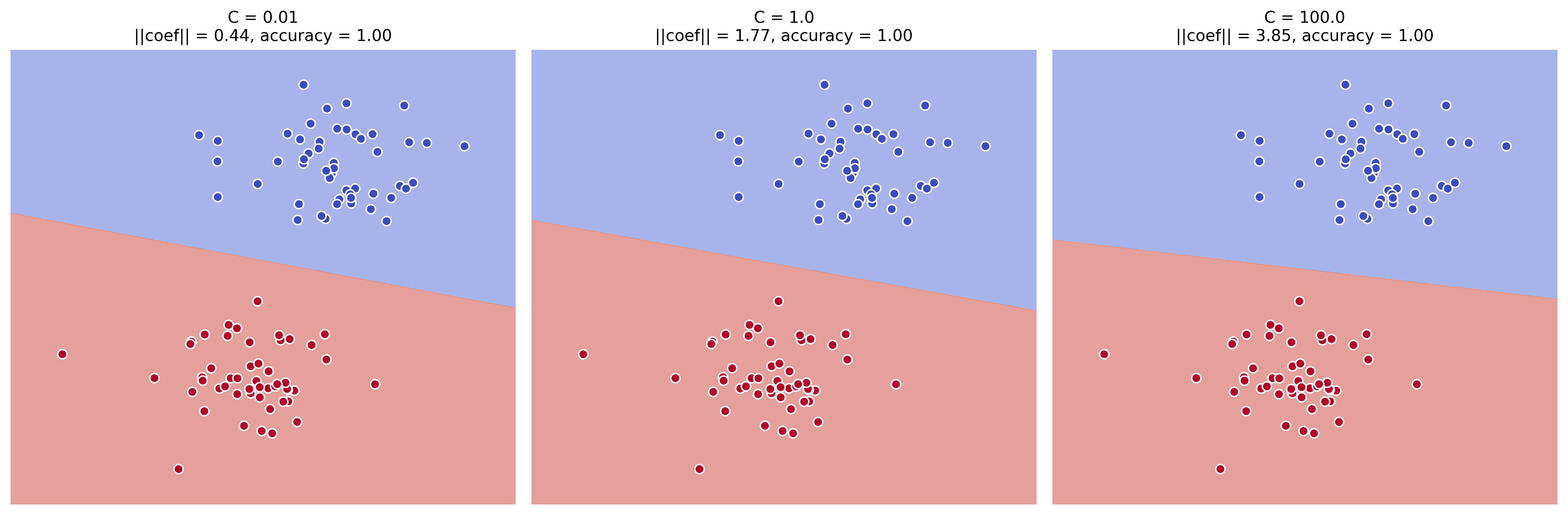
All three reach the same accuracy on this easily-separable toy dataset, but the learned weight vector's magnitude grows substantially as C increases from 0.01 to 100, 0.44 up to 3.85, exactly the shrink-toward-zero behavior regularization is supposed to produce, weaker regularization (higher C) lets the weights grow larger and the boundary fit the training points more tightly.

2. Solvers: How the Loss Actually Gets Minimized

Ch.24 minimized log loss with plain gradient descent, computed and coded by hand. scikit-learn's solver parameter picks between five different, more sophisticated optimization algorithms for doing that same minimization: 'newton-cg', 'lbfgs', 'liblinear', 'sag', 'saga'. Each one is a different numerical strategy with its own trade-offs (memory use, convergence speed, dataset size it scales to), not something this series derives from scratch, but the one detail worth remembering is that not every solver supports every penalty:

saga is the only solver that supports every penalty type, including elasticnet, and liblinear is the odd one out that doesn't support None (no regularization) at all. The default, lbfgs, handles the common l2-or-None case fine without ever needing to be changed; solver only needs deliberate attention when switching to l1 or elasticnet.

3. Convergence: max_iter and tol

max_iter is the same idea as the epochs loop bound from Ch.24's from-scratch gradient descent, an upper limit on how many optimization steps the solver takes before giving up, default 100. Every ConvergenceWarning that's shown up quietly in this series' own code output whenever a solver ran on real data traces back to this exact parameter, the fix is almost always to raise max_iter, not to change anything else. tol sets the actual stopping threshold the solver checks against internally (how small a loss improvement counts as "converged"), it's rarely touched directly, raising max_iter is the more common fix when a model isn't converging.

4. Multi-Class Strategy: multi_class

This one maps directly onto Ch.28. multi_class accepts 'ovr', 'multinomial', or 'auto':

• 'ovr' is Ch.28 Section 2's naive intuition-building approach, one-vs-rest, a separate binary Logistic Regression model trained per class.
• 'multinomial' is real softmax regression, Ch.28 Sections 4 through 8, one joint model trained against the multinomial loss.
• 'auto' (the default) picks 'multinomial' whenever the chosen solver supports it, which is the generally better-performing option, and falls back to 'ovr' otherwise. Leaving this on 'auto' is the right call almost always.

5. Everything Else, Briefly

The remaining parameters are rarely worth touching, but each has a specific, narrow purpose:

• fit_intercept (default True): whether to learn $w_0$ at all. Leave it on.
• class_weight (default None): set to 'balanced' on an imbalanced dataset (the exact problem Ch.25's terrorist-detection example ran into) to reweight the loss so the minority class isn't ignored.
• random_state: seeds the randomness used internally by the sag, saga, and liblinear solvers; irrelevant for the others.
• dual (default False): switches between the primal and dual optimization formulation, only relevant with solver='liblinear' and penalty='l2' when there are more features than rows; leave it False otherwise.
• warm_start (default False): if True, calling .fit() again continues from the previously learned weights instead of restarting from scratch, useful when refitting the same model repeatedly with slightly different data.
• n_jobs: parallelizes training across CPU cores, but only actually helps when multi_class='ovr', since that's the one case training genuinely splits into independent per-class jobs that can run at once.
• verbose: prints solver progress during training, a debugging aid, not something that changes model behavior.

6. The Practical Takeaway

Most of the time, the defaults (penalty='l2', C=1.0, solver='lbfgs', multi_class='auto') are a fine starting point. The two worth actively tuning on a real problem are C (search across a log-spaced range, like 0.001, 0.01, 0.1, 1, 10, 100, checking cross-validated accuracy at each) and class_weight='balanced' when the dataset is imbalanced. solver only needs a deliberate choice when penalty is set to 'l1' or 'elasticnet', and everything else is best left alone until there's a specific, concrete reason to change it.

That's the full arc: from the perceptron trick's step function in Ch.20 to a working understanding of every dial scikit-learn's LogisticRegression exposes.