Ch.29: Fitting Non-Linear Data With Polynomial Logistic Regression

Inspired by: YouTube

Since Ch.20, every Logistic Regression example in this series has assumed the two classes are separable by a straight line. Real data often isn't. This post covers a trick that lets plain Logistic Regression handle non-linear data anyway, by reusing an idea already covered for Polynomial Regression.

1. Why Logistic Regression Fails on Non-Linear Data

Logistic Regression's decision boundary, everywhere its raw score $z = w_1x_1 + w_2x_2 + \dots + w_0$ crosses 0, is always a straight line (or, with more features, a flat hyperplane). That's a direct consequence of $z$ being a linear combination of the input features. If the two classes in a dataset genuinely can't be separated by any straight line, no choice of weights fixes that, the model architecture itself is the bottleneck.

The usual advice at that point is to reach for a different algorithm entirely, Decision Trees, Random Forest, SVM, algorithms whose decision boundaries aren't restricted to straight lines. Those get covered later in this series. But there's a way to stretch Logistic Regression itself to fit curved boundaries first.

2. Borrowing Polynomial Regression's Trick

Ch.11 covered the same underlying problem for regression: plain Linear Regression can only fit a straight line, but running PolynomialFeatures on the input columns before fitting lets the same linear model trace a curve, because the curve is linear in the transformed, higher-degree feature space even though it's curved in the original one.

The identical trick applies to Logistic Regression. For a 2-column dataset ($x_1$, $x_2$) and a chosen degree, say 2, PolynomialFeatures expands those two columns into six: 1, $x_1$, $x_2$, $x_1^2$, $x_1 x_2$, $x_2^2$ (bias, the two original linear terms, and every quadratic combination). Fitting Logistic Regression on those six columns still draws a straight decision boundary, but in six-dimensional space. Projected back down onto the original two input dimensions, that flat boundary appears curved, because it's now a function of $x_1^2$, $x_1x_2$, and $x_2^2$, not just $x_1$ and $x_2$ directly. Raising the degree further keeps adding higher-order terms ($x_1^3$, $x_1^2x_2$, and so on), letting the boundary bend more.

3. Applying It

from sklearn.preprocessing import PolynomialFeatures
from sklearn.linear_model import LogisticRegression
 
poly = PolynomialFeatures(degree=3)
X_trf = poly.fit_transform(X)
 
clf = LogisticRegression()
clf.fit(X_trf, y)

Nothing about LogisticRegression itself changes, only the data it sees. The transform happens once, up front; from the model's point of view it's still fitting an ordinary straight-line boundary, just in an expanded feature space, exactly like Ch.11's version of this trick.

4. On a Genuinely Non-Linear Dataset

Testing this on a toy dataset shaped so that no straight line can separate its two classes well, following the source notebook:

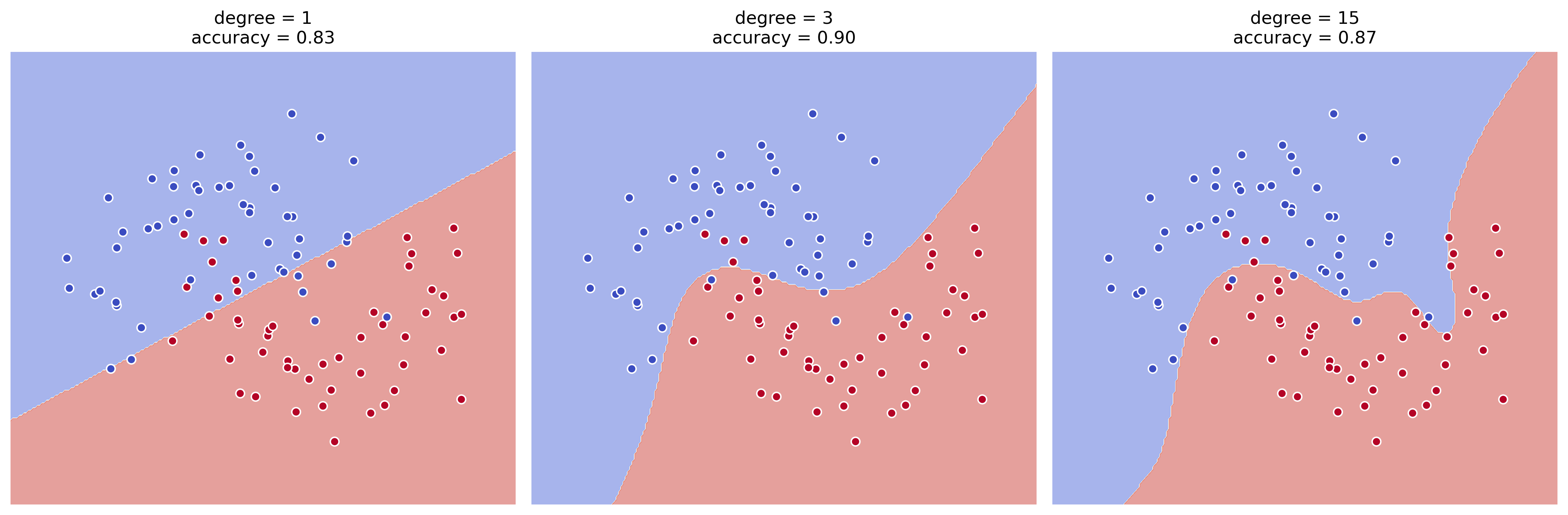
Plain Logistic Regression (degree=1, no transform) draws a single straight line and gets 10-fold cross-validated accuracy of 0.83, visibly misclassifying a cluster of points sitting right where the true boundary curves away from a straight line. Applying PolynomialFeatures(degree=3) first raises accuracy to 0.90, and the plotted boundary now visibly bends to follow the data's actual shape instead of cutting straight through it.

5. Degree Is Just Another Complexity Knob

Pushing the degree further doesn't keep helping. At degree=15, accuracy actually drops to 0.87, below the degree=3 result, and the boundary in the plot turns visibly jagged, chasing individual outlier points with sharp little detours instead of following the data's overall shape. That's the exact same bias-variance story covered in Ch.12: too low a degree underfits (a straight line can't capture a curved boundary), too high a degree overfits (the model starts memorizing noise instead of the underlying pattern), and somewhere in between, here around degree=3 to 5, sits the sweet spot that generalizes best. Degree is a hyperparameter like any other, worth sweeping across a small range and checking cross-validated accuracy at each value rather than guessing.

6. Should This Actually Be Used?

Worth being direct about this technique's real-world standing: in practice, on genuinely non-linear datasets, algorithms whose decision boundaries aren't artificially built out of polynomial terms, Decision Trees and Random Forest especially, tend to outperform this approach and need far less hand-tuning of a degree parameter. Polynomial Logistic Regression is worth knowing because it's a direct, useful extension of ideas already covered (Ch.11's polynomial features, Ch.12's under/overfitting trade-off), and it's a fully legitimate option when Logistic Regression specifically is required for other reasons. But it's rarely the first tool reached for on non-linear data once tree-based algorithms are available, which this series covers next.