Ch.13: Ridge Regression: Regularization and the L2 Penalty

Inspired by: YouTube

In the previous post on the Bias-Variance Tradeoff, we established that as model complexity increases, training error drops toward zero while variance can explode. The post concluded by noting that to combat high variance without sacrificing model simplicity, we need a mechanism to constrain model parameters.

That mechanism is Regularization.

1. What Is Regularization, and Where Do We Use It

Regularization is a technique where we deliberately inject additional information into a model's optimization process so that it stops chasing every point in the training set and generalizes better to unseen data.

It sits alongside two other well known techniques for fighting overfitting: bagging and boosting. Bagging trains many models on bootstrapped samples and averages them, boosting builds models sequentially to correct earlier errors, and regularization takes a different route entirely: it changes the loss function itself so that large, unstable coefficients get penalized during training. It is especially relevant to regression, linear regression, logistic regression, and any model built on top of a perceptron.

There are three regularized linear models, distinguished by the penalty they add to the loss function:

1. Ridge Regression (L2 Regularization): Adds a penalty proportional to the sum of squared coefficient magnitudes ($\sum w_j^2$). This is the subject of this post.
2. Lasso Regression (L1 Regularization): Adds a penalty proportional to the sum of absolute coefficient values ($\sum |w_j|$).
3. ElasticNet Regression: Combines both L1 and L2 penalties into a single joint objective function.

2. Why Overfitting Shows Up as Large Coefficients

The whole idea of linear regression is to find the best fit line, $y = mx + b$. Left unconstrained, the standard Ordinary Least Squares (OLS) loss only cares about minimizing the error on the training points:

$L = \sum_{i=1}^n \left(y_i - \hat{y}_i\right)^2$

Nothing in this expression restricts how large the slope $m$ (or, in multiple regression, the weights $w_j$) is allowed to get. Given a training set with only a couple of points, or noisy points that do not sit on a clean line, OLS is happy to tilt the line as steeply as needed to pass through every single one of them, driving the slope higher and the training error toward zero. That is overfitting from the model's perspective: a high value of $m$ that fits the training data almost perfectly but has no reason to hold up on data it has not seen. Underfitting is the mirror image: the slope is pushed toward zero and the line stops responding to the data at all.

A Concrete Whiteboard Example

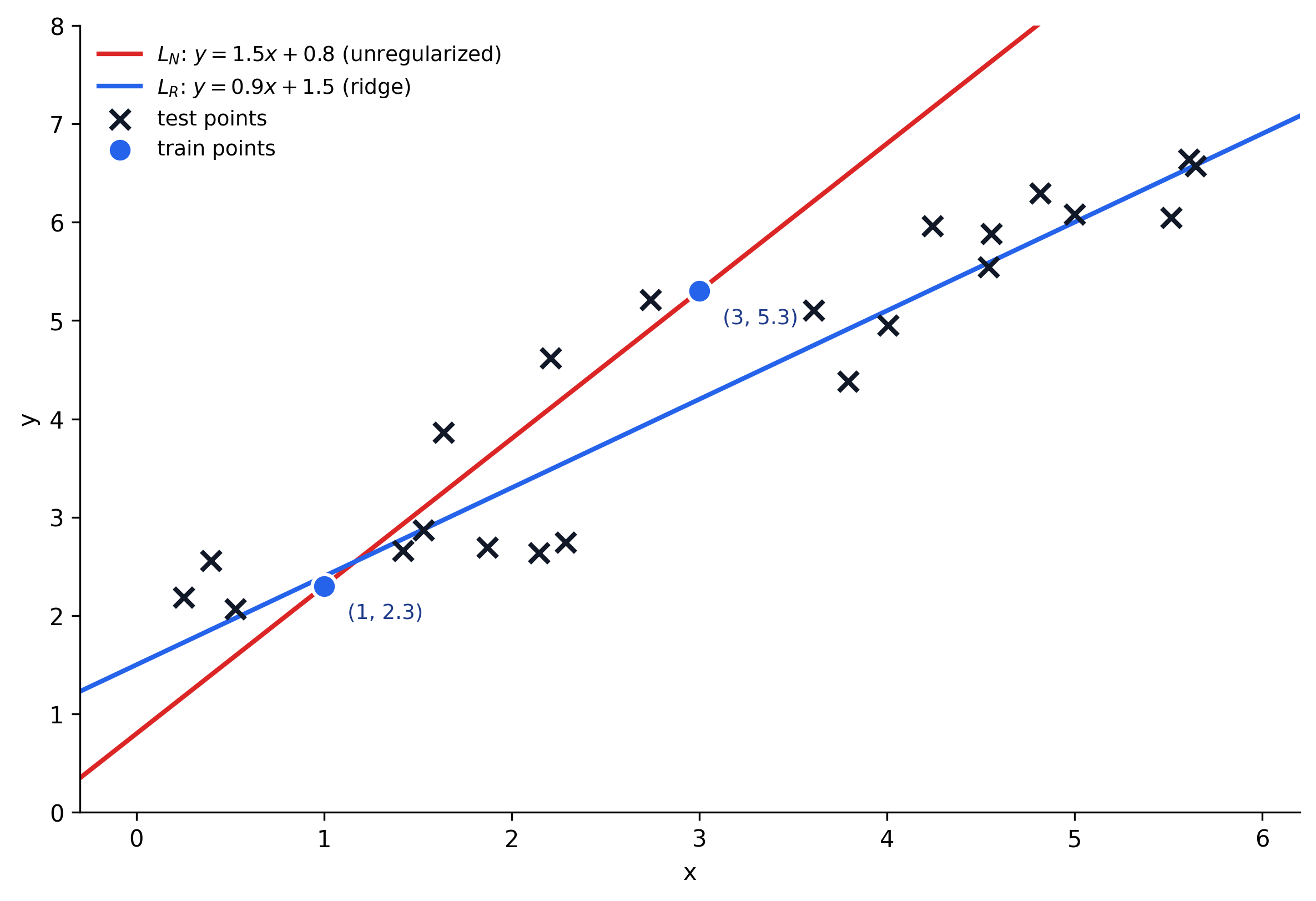
Here is the example used to make this tangible. Take two training points, drawn as the blue dots:

$(1,\ 2.3) \quad \text{and} \quad (3,\ 5.3)$

Two candidate lines are fit to them:

• $L_N$: $y = 1.5x + 0.8$, an unregularized line that passes through both training points exactly.
• $L_R$: $y = 0.9x + 1.5$, a shallower, regularized line that misses both points by a small margin.

The rest of the plot is a cloud of test points, marked as crosses, sitting further out and slightly off the trajectory the training points suggest. That gap between the two training dots and the crosses is deliberate: it is there to show what happens when a line is tuned tightly to only two points and then asked to predict a wider, noisier population. $L_N$, having been pulled steeply through the training pair, drifts away from the cross cluster. $L_R$, with its gentler slope, tracks the cross cluster far more closely even though it does not touch either training point exactly.

Computing the plain OLS loss on the two training points for each line:

$L(L_N) = (2.3 - 2.3)^2 + (5.3 - 5.3)^2 = 0$

$L(L_R) = (2.3 - 2.4)^2 + (5.3 - 4.2)^2 = 0.01 + 1.21 = 1.22$

Judged purely on training error, $L_N$ wins with a perfect score of $0$ against $L_R$'s $1.22$. This is exactly the problem: OLS alone always prefers the steeper line, because nothing in the loss punishes the slope for being large.

3. Adding the Penalty Term

Ridge Regression fixes this by appending a penalty on the slope directly into the loss:

$L = \sum_{i=1}^n \left(y_i - \hat{y}_i\right)^2 + \lambda m^2$

With $\lambda = 1$, recompute the total loss for both lines, this time including $\lambda m^2$:

$L(L_N) = 0 + 1 \times (1.5)^2 = 0 + 2.25 = 2.25$

$L(L_R) = 1.22 + 1 \times (0.9)^2 = 1.22 + 0.81 = 2.03$

The ranking flips. $L_N$ had a flawless training fit but its steep slope now costs it $2.25$ in total loss. $L_R$ gave up a little training accuracy but its gentler slope keeps its total loss lower, at $2.03$. Ridge Regression picks $L_R$, and by extension, the line that generalizes better to the cross-marked test points, precisely because the $\lambda m^2$ term makes a large slope expensive even when it fits the training data perfectly.

In multiple linear regression this generalizes from a single slope $m$ to the full weight vector, and the penalty becomes $\lambda \sum_{j=1}^p w_j^2$. That $\lambda$ is exposed to us as a tunable hyperparameter, alpha in Scikit-Learn, and how it trades off bias against variance is worth its own post.