Ch.28: Softmax Regression for Multi-Class Classification

By Ayush Arora•2026-08-29•7 min read

Inspired by: YouTube

Every Logistic Regression post so far, Ch.20 through Ch.24, assumed exactly two classes. But the student placement dataset used throughout this series actually has a third outcome: a student can get placed, not get placed, or sit out of placements entirely (higher studies, entrepreneurship, and so on). Binary Logistic Regression has no way to handle three classes at once. This post covers the extension that does: softmax regression, also called multinomial Logistic Regression.

1. The Softmax Function

Binary Logistic Regression uses sigmoid to turn one raw score into one probability. Softmax generalizes that idea to $K$ classes at once: given $K$ raw scores $z_1, \dots, z_K$ (one per class), it converts them into $K$ probabilities that all sum to $1$ :

\sigma(z_j) = \frac{e^{z_j}}{\sum_{k=1}^{K} e^{z_k}}

For the placement example, $K=3$ : $z_1$ for "placed," $z_2$ for "not placed," $z_3$ for "sat out." Plugging each into the formula above gives $P(\text{placed})$ , $P(\text{not placed})$ , and $P(\text{sat out})$ , three numbers that add up to exactly $1$ , exactly like sigmoid's output and its complement summed to $1$ in the binary case. In fact, softmax with $K=2$ reduces algebraically to plain sigmoid, binary Logistic Regression is just softmax regression's two-class special case, not a separate technique.

2. Building the Intuition: One Model Per Class

Before seeing how real softmax regression trains, it helps to build the intuition the naive way (this isn't what scikit-learn actually does internally, it's a stepping stone).

Start by one-hot encoding the output column: instead of one placement column with three possible values, make three binary columns, is_placed, is_not_placed, is_sat_out, each 1 exactly where that outcome occurred and 0 everywhere else. That turns one 3-class problem into three separate binary classification problems, each with the same CGPA/IQ input columns:

Dataset 1: CGPA, IQ → is_placed (1 or 0)
Dataset 2: CGPA, IQ → is_not_placed (1 or 0)
Dataset 3: CGPA, IQ → is_sat_out (1 or 0)

Train three completely independent binary Logistic Regression models, one per dataset. Each one learns its own weights, Model 1 learns $w_1, w_2, w_0$ for "placed vs. everything else," and likewise for Models 2 and 3, nine weights total for two input features and three classes.

3. Predicting With Three Models

For a new student, compute a raw score from each of the three trained models:

z_1 = w_1^{(1)}\cdot\text{CGPA} + w_2^{(1)}\cdot\text{IQ} + w_0^{(1)}, \quad z_2 = \ldots, \quad z_3 = \ldots

Then run all three scores through the softmax formula from Section 1 together, so the three resulting probabilities are properly normalized against each other, and assign the class with the highest probability. Three independently-trained binary models, combined at prediction time through one shared softmax step.

4. Why This Doesn't Scale

Training $K$ completely independent models works, but it's slow, especially as the dataset grows: every one of the $K$ models runs its own full gradient descent loop over the entire training set. With a large dataset and many classes, that's $K$ times the training cost of one model.

The actual softmax regression algorithm avoids this by changing the loss function itself instead of the number of models. A single joint model gets trained by one gradient descent run, and that one run produces weights for all $K$ classes simultaneously, no separate per-class training loops required.

5. The Multinomial Loss Function

Binary Logistic Regression's log loss from Ch.23 was:

L = -\frac{1}{m}\sum_{i=1}^{m}\Big[y_i\log(\hat y_i) + (1-y_i)\log(1-\hat y_i)\Big]

Softmax regression's version generalizes this from two terms per row to $K$ terms per row, one for every class, using one-hot encoded labels $y_{ik}$ (which is $1$ if row $i$ truly belongs to class $k$ , else $0$ ) and softmax's per-class predicted probabilities $\hat y_{ik}$ :

L = -\frac{1}{m}\sum_{i=1}^{m}\sum_{k=1}^{K} y_{ik}\log(\hat y_{ik})

The outer sum runs over every training row, exactly as before. The inner sum runs over every class for that row, this is the new part.

6. Why the Inner Sum Collapses to One Term

That double sum looks more intimidating than it actually is, because $y_{ik}$ is one-hot: for any given row, it's 1 for exactly one class and 0 for every other class. Take a tiny 3-row, 3-class dataset with one-hot labels:

Row	$y_{i1}$	$y_{i2}$	$y_{i3}$
1	1	0	0
2	0	0	1
3	0	1	0

For row 1, the inner sum is $y_{11}\log(\hat y_{11}) + y_{12}\log(\hat y_{12}) + y_{13}\log(\hat y_{13})$ . Since $y_{12}=0$ and $y_{13}=0$ , those two terms vanish entirely (anything times 0 is 0), leaving just $y_{11}\log(\hat y_{11}) = \log(\hat y_{11})$ . The same happens for every row: whichever class is the true label is the only term that survives, everything else zeroes out. So the full loss for this dataset is just:

L = -\frac{1}{3}\Big[\log(\hat y_{11}) + \log(\hat y_{23}) + \log(\hat y_{32})\Big]

One log-probability term per row, the predicted probability the model assigned to that row's actual class, exactly the same intuition as binary log loss, just picking out one of $K$ terms per row instead of one of $2$ .

7. Parameter Count and Gradient Descent

With $K$ classes and $n$ input features, softmax regression has $K \times (n+1)$ total parameters, $n$ weights plus one intercept, per class. For the 2-feature, 3-class placement example, that's $3 \times 3 = 9$ weights total, the same nine numbers Section 2's three separate models produced, but now all learned from a single gradient descent run against the one loss function in Section 5, instead of three independent training loops.

8. Softmax Regression For Real

scikit-learn's LogisticRegression handles softmax regression directly, no separate class needed, following the source notebook:

from sklearn.linear_model import LogisticRegression
 
clf = LogisticRegression(multi_class="multinomial")
clf.fit(X_train, y_train)

Running this on the Iris dataset (sepal length and petal length as the two input features, three species as the three classes):

from sklearn.metrics import accuracy_score
 
y_pred = clf.predict(X_test)
print(accuracy_score(y_test, y_pred))
 
query = np.array([[3.4, 2.7]])
print(clf.predict_proba(query))

This gives 96.7% accuracy on the test split, and for a new flower with sepal length 3.4 and petal length 2.7, predict_proba returns [0.726, 0.274, 0.0004], a 72.6% probability of setosa, 27.4% versicolor, and a virtually nonexistent 0.04% chance of virginica. Softmax assigns the class with the highest probability, setosa here, exactly the argmax step from Section 3, just computed by one trained model instead of three.

Plotting the model's decision regions across the two input features shows all three classes carved out at once:

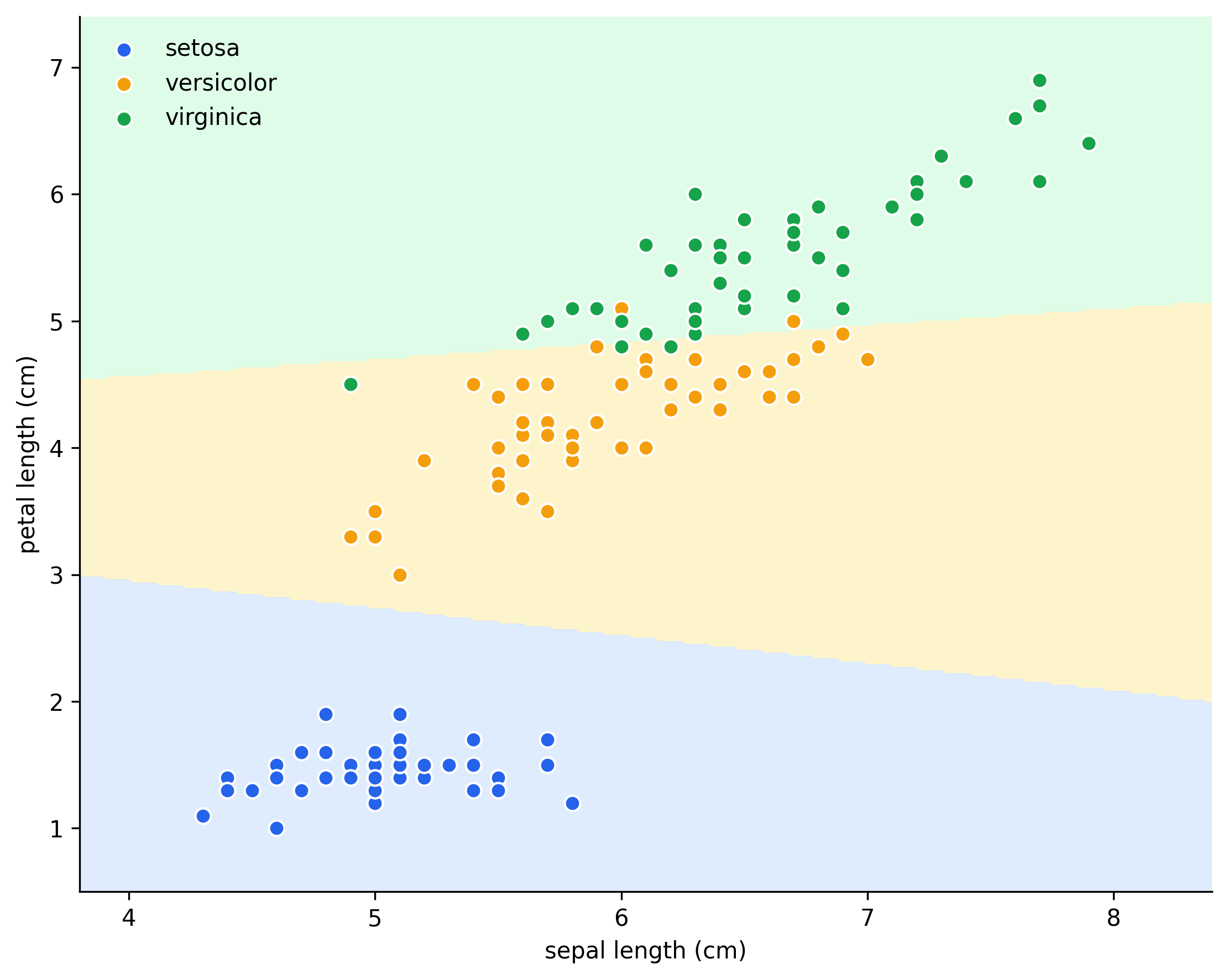
Scatter plot of Iris flowers by sepal length and petal length, colored by species: blue setosa points cluster in the bottom-left, orange versicolor in the middle, green virginica in the upper-right. The background is shaded into three regions, light blue, light yellow, light green, by which class the softmax model predicts there, with two nearly straight boundary lines separating them

Two boundary lines split the plane into three regions, one per class, the direct multi-class generalization of the single boundary line a binary Logistic Regression draws.

9. What's Left

This post covered softmax regression's intuition and its end-to-end use through scikit-learn, without deriving the gradient descent update rule for the multinomial loss from Section 5, the same next step Ch.24 took for the binary case. That derivation, and coding a from-scratch multinomial classifier the way Ch.24 did for the binary one, is naturally where this thread picks back up.

View all chapters in Machine Learning Algorithms →