Ch.25: Accuracy, the Confusion Matrix, and Why Accuracy Lies

By Ayush Arora•2026-08-27•8 min read

Inspired by: YouTube

Ch.20 through Ch.24 built Logistic Regression, a classification algorithm, from scratch. The regression posts earlier in this series had regression metrics (R², adjusted R²) to answer "how good is this model?" Classification needs its own equivalent. This post covers the simplest one, accuracy, and the problem that makes it dangerous to trust blindly.

1. Accuracy: The Basic Idea

Take a familiar toy setup: a dataset of students, each with a CGPA, an IQ, and whether they got placed. Split it into 800 training rows and 200 test rows, train two classifiers (Logistic Regression and a Decision Tree) on the training set, and run both on the 200 test rows.

For every test row, there's an actual outcome (did the student get placed or not) and a predicted outcome (what the model guessed). Accuracy asks one question per row: did the prediction match reality? Then it counts:

\text{accuracy} = \frac{\text{number of correct predictions}}{\text{total number of predictions}}

If a model gets 8 out of 10 predictions right, its accuracy is $0.8$ , or 80%. That's the entire idea, nothing more subtle than "how often was it right."

2. Computing It for Real

Running this on the UCI heart disease dataset (each row is a patient's clinical measurements, target is whether they have heart disease), following the source notebook:

from sklearn.model_selection import train_test_split
from sklearn.linear_model import LogisticRegression
from sklearn.tree import DecisionTreeClassifier
from sklearn.metrics import accuracy_score, confusion_matrix
 
X_train, X_test, y_train, y_test = train_test_split(
    df.iloc[:, 0:-1], df.iloc[:, -1], test_size=0.2, random_state=2
)
 
clf1 = LogisticRegression()
clf2 = DecisionTreeClassifier()
clf1.fit(X_train, y_train)
clf2.fit(X_train, y_train)
 
y_pred1 = clf1.predict(X_test)
y_pred2 = clf2.predict(X_test)
 
print(accuracy_score(y_test, y_pred1))  # Logistic Regression
print(accuracy_score(y_test, y_pred2))  # Decision Tree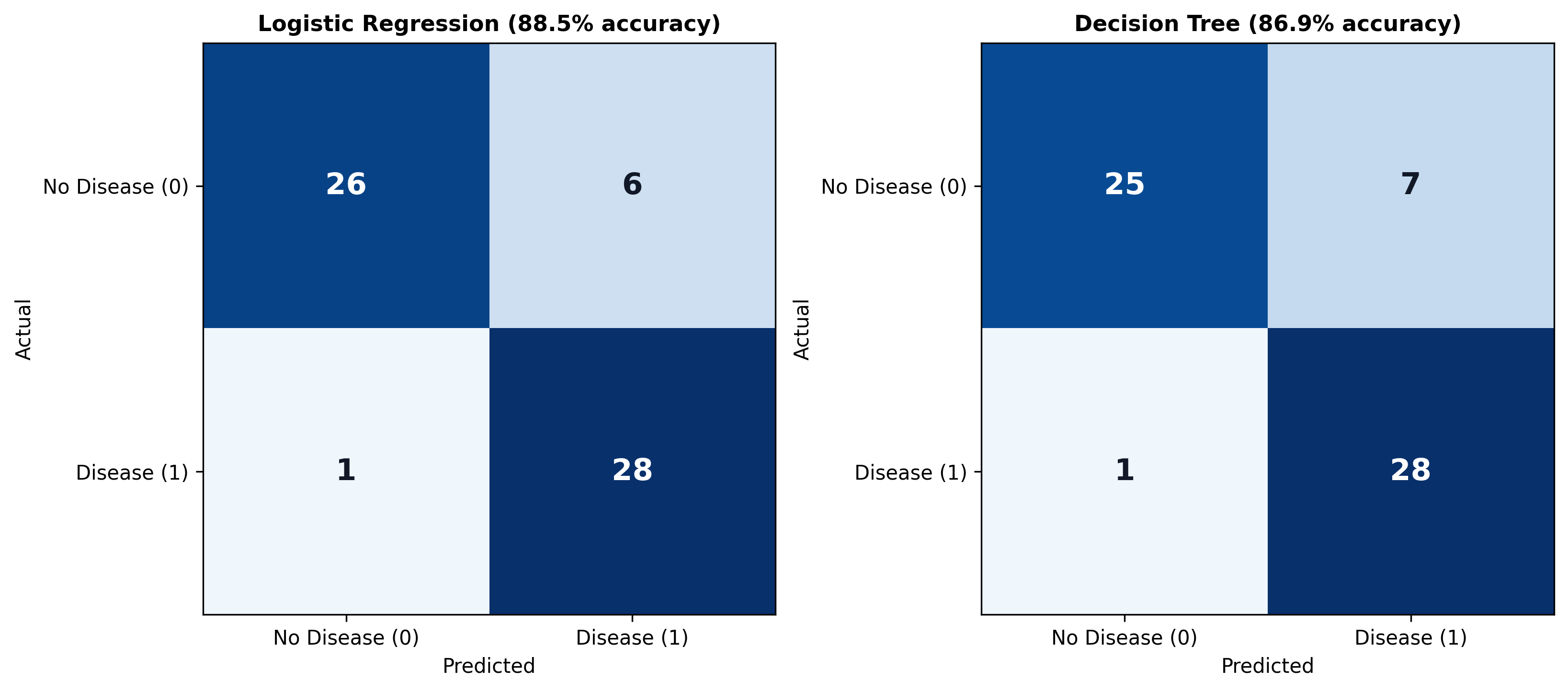

Two side-by-side 2x2 heatmap confusion matrices for the heart disease dataset. Logistic Regression (88.5% accuracy): 26 true negatives, 6 false positives, 1 false negative, 28 true positives. Decision Tree (86.9% accuracy): 25 true negatives, 7 false positives, 1 false negative, 28 true positives

Logistic Regression comes out at 88.5% accuracy, the Decision Tree at 86.9%, so on this split, Logistic Regression is the better model. Note this generalizes to more than two classes without any change in logic, on a 3-class problem like Iris or a 10-class problem like MNIST digits, accuracy is still just correct predictions divided by total predictions, counted the same way.

3. How High Should Accuracy Be?

There's a tempting instinct to treat a higher accuracy number as always better, and to want a single target number to aim for, "accuracy should be at least X%." That instinct is wrong. There's no universal threshold, it depends entirely on what the model is used for and what a mistake costs.

Take a model that screens chest X-rays for cancer at 99% accuracy. That sounds excellent, but it means that out of 100 patients, the model is wrong about one. A missed cancer diagnosis can cost a life, so 99% is not nearly good enough to deploy in that setting, no hospital would accept it. The same 99% is also unacceptable for a self-driving car deciding whether to steer left or right, a wrong call once every hundred decisions on a real road is a serious accident waiting to happen.

Contrast that with a model predicting whether a particular customer will order food from a restaurant this weekend, based on their past month's behavior. An 80% accurate model here is perfectly fine to ship, a wrong prediction just means a slightly less-targeted notification, not a life-or-death outcome. So the honest answer to "how much accuracy is enough" is always: it depends on the problem being solved and the cost of getting it wrong, there is no fixed correct number.

4. Where Accuracy Falls Short

Accuracy compresses everything into a single number: 90% accuracy means the model is wrong 10% of the time. But it doesn't say what kind of wrong. In a binary classification problem, a mistake can happen in two different directions:

A patient truly has heart disease, but the model says they don't.
A patient truly doesn't have heart disease, but the model says they do.

These two mistakes are not equally costly, missing a real diagnosis is far worse than a false alarm that gets ruled out on further testing, but accuracy treats both as identical "wrong" and blends them into one percentage. To see the two error types separately, a different tool is needed: the confusion matrix.

5. The Confusion Matrix and Its Four Cells

A confusion matrix is a small grid: for binary classification, a 2×2 table, with actual labels on one axis and predicted labels on the other. Each of its four cells has a name:

True Positive (TP): predicted positive, and it actually was positive.
False Positive (FP): predicted positive, but it actually was negative.
False Negative (FN): predicted negative, but it actually was positive.
True Negative (TN): predicted negative, and it actually was negative.

A tip for remembering which word means what: the second word, "Positive" or "Negative," always comes from the prediction. The model predicted 1, call it positive; the model predicted 0, call it negative. The first word, "True" or "False," then says whether that prediction matched the actual value: True if the prediction was correct, False if it wasn't. So a False Positive is a case the model called positive, and was wrong to; a False Negative is a case the model called negative, and was wrong to.

Read back the heart disease confusion matrix above with this rule: Logistic Regression's grid has 28 true positives (correctly caught disease), 26 true negatives (correctly cleared healthy patients), 6 false positives (healthy patients incorrectly flagged), and 1 false negative (a diseased patient the model missed). That last cell is exactly the kind of mistake accuracy alone would hide inside a single 88.5% figure.

Accuracy can always be recovered from the confusion matrix, it's just the diagonal (correct cells) over the total:

\text{accuracy} = \frac{TP + TN}{TP + TN + FP + FN}

but the reverse doesn't work, accuracy alone can't tell you the four individual cell counts. That's the whole reason the confusion matrix exists: it keeps information accuracy throws away. This generalizes past 2×2 too, an $n$ -class problem produces an $n \times n$ confusion matrix, still with correct predictions running along the diagonal.

6. Type I and Type II Errors

The two off-diagonal cells have standard names that come up constantly in interviews:

False Positive = Type I error.
False Negative = Type II error.

For the heart disease model, a Type I error is telling a healthy patient they have heart disease, an unnecessary scare and probably some unnecessary follow-up tests. A Type II error is telling a genuinely sick patient they're fine, a missed diagnosis with real consequences. Neither type is universally "the worse one," which error matters more depends entirely on the problem, exactly like the accuracy threshold question in Section 3.

7. Why Accuracy Can Actively Mislead: Imbalanced Datasets

Accuracy's real danger shows up on imbalanced datasets, where one class vastly outnumbers the other. Consider building a model for airport security that scans passenger photos and predicts whether someone is a potential terrorist. In the real world, this is an extreme imbalance: out of, say, a million passengers, maybe one is actually a threat, the other 999,999 are completely ordinary travelers.

Now imagine a deliberately useless model: it never looks at the photo at all, and just always predicts "not a terrorist" for everyone. Out of a million passengers, it's wrong exactly once, on the one actual terrorist it waves through. Its confusion matrix looks like this:

TP = 0 (it never predicts "terrorist," so it can never be right about one)
FN = 1 (the one real terrorist, incorrectly waved through)
FP = 0 (it never predicts "terrorist," so no false alarms either)
TN = 999,999 (every ordinary passenger, correctly cleared)

\text{accuracy} = \frac{TP+TN}{TP+TN+FP+FN} = \frac{0 + 999{,}999}{0+999{,}999+0+1} = 99.9999\%

A model that does nothing but say "not a terrorist" every single time scores essentially perfect accuracy, and is also completely useless, it has a 100% failure rate at the one job it exists to do. If accuracy were relied on here to judge the model, this do-nothing model would look outstanding. That's the trap: on an imbalanced dataset, accuracy can be dominated entirely by how well the model handles the majority class, while telling nothing about performance on the minority class that actually matters.

This is why accuracy isn't always the right metric, especially for imbalanced problems, and it's what motivates two more classification metrics built directly on top of the confusion matrix's TP/FP/FN/TN cells: precision and recall. Those are next.

View all chapters in Machine Learning Algorithms →