
Ch.20: Logistic Regression: The Perceptron Trick
Inspired by: YouTube
This closes out linear regression's regularization arc (Ch.13 through Ch.19) and starts a new topic: Logistic Regression, a classification algorithm despite the name, and one of the most foundational in machine learning. Understanding it well is also a good stepping stone toward neural networks, since the perceptron, deep learning's basic building block, is barely different from it.
This post covers the geometric intuition first, through an algorithm called the Perceptron Trick, before the probability-based math behind actual Logistic Regression in a later post.
1. The Requirement: (Almost) Linearly Separable Data
Logistic Regression draws a straight line (or in higher dimensions, a hyperplane) to separate two classes. Picture a dataset of students, CGPA on one axis, IQ on the other, colored by whether they got placed:
Data like this, where a single straight line can cleanly separate the two colors, is called linearly separable. It doesn't have to be perfect, a couple of stray points on the wrong side is fine, that's almost linearly separable and still works well in practice. What doesn't work is genuinely nonlinear data, concentric circles of two classes, for instance, where no straight line, no matter how it's drawn, ever separates the two groups:
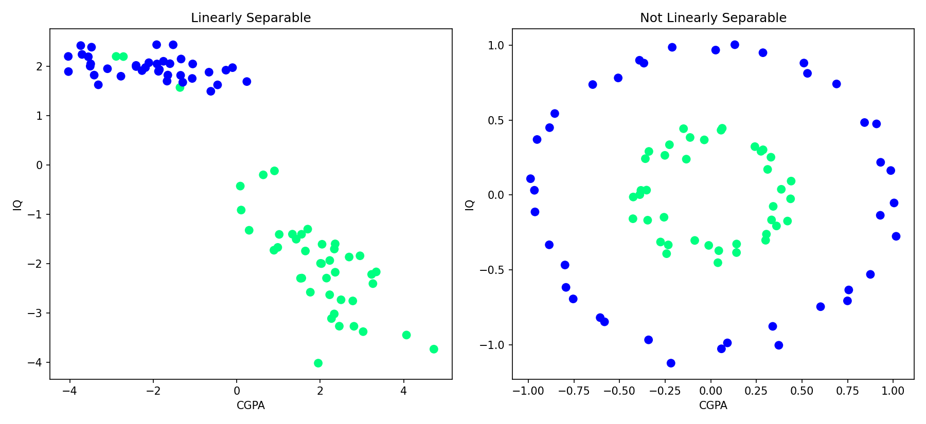
Logistic Regression, like linear regression, only ever draws a straight line (or flat hyperplane), so nonlinear data like the ring on the right needs a different tool entirely.
2. The Line's Equation, Written a Different Way
Linear regression writes a line as . Classification never uses that form, it breaks down as soon as the line is vertical. Instead, the line is written in general form:
In three dimensions this becomes a plane, , and in higher dimensions still, a hyperplane, just with more terms added the same way.
3. Finding Which Side of the Line a Point Is On
Given the line's equation and any point's coordinates, plugging the coordinates into tells you which side it's on:
- Result : the point is on the positive side.
- Result : the point is on the negative side.
- Result : the point sits exactly on the line.
For the line , plugging in a point like gives , positive side. Flip the line's sign, , and the same point now evaluates to , negative side, since the entire line's positive and negative regions swap along with the sign.
4. How the Line Moves: Rotation and Translation
A line's shape is entirely controlled by its three coefficients , , , and each one moves the line differently:
- Changing translates the line up or down without changing its angle. Increase and the line shifts down; decrease it and the line shifts up.
- Changing or rotates the line around a fixed point, tilting it one way or the other depending on which coefficient changes and by how much.
Combine changes to all three and the line both rotates and translates at once, exactly the kind of move needed to steer a line toward a point it's currently misclassifying.
5. The Perceptron Trick
The algorithm's core idea is almost embarrassingly simple:
- Start with a random line (random , , ).
- Loop for a fixed number of iterations (or until convergence).
- On each iteration, pick a random point from the training data.
- Ask that point: are you on the correct side of the line?
- If yes, do nothing.
- If no, nudge the line toward that point.
Repeat that enough times and the line gradually rotates and slides into a position that separates the two classes. The nudge itself follows a simple rule: if a point that should be negative is stuck in the positive region, subtract that point's coordinates (scaled down) from the line's coefficients; if a point that should be positive is stuck in the negative region, add them. Either direction pulls the line toward the misclassified point until it lands on the correct side.
That "scaled down" part matters: nudges are never applied at full strength in one step, that would send the line flying past a reasonable position. Instead each nudge is scaled by a small constant called the learning rate, typically something like 0.01 or 0.1, the same idea gradient descent uses in Ch.7.
6. Writing the Line as a Weight Vector
To make this codeable, the line's coefficients get renamed into a weight vector: , , . A line in two dimensions becomes:
Prepending a constant column of 1s to the input data (the same trick Ch.14 used for the intercept) turns this into one clean dot product:
Predicting a new point's class is now just: compute , and if the result is predict the positive class, otherwise predict the negative class.
7. One Update Rule Instead of Two
The two-case rule from step 5 (add for a positive point stuck negative, subtract for a negative point stuck positive) can be collapsed into a single formula. Let be the model's current prediction (1 or 0) and be the actual label (1 or 0):
Checking all four possible combinations of actual label and prediction confirms this reduces correctly:
| Actual | Predicted | Update | |
|---|---|---|---|
| 1 (placed) | 1 (placed) | 0 | No change, correctly classified |
| 0 (not placed) | 0 (not placed) | 0 | No change, correctly classified |
| 1 (placed) | 0 (not placed) | 1 | , a positive point stuck negative gets pulled up |
| 0 (not placed) | 1 (placed) | -1 | , a negative point stuck positive gets pulled down |
Both correct-classification cases naturally zero out the update, and both misclassification cases naturally reproduce the add/subtract rule from before, without ever needing an explicit if branch for which direction to nudge.
8. Implementing It From Scratch
import numpy as np
from sklearn.datasets import make_classification

X, y = make_classification(n_samples=100, n_features=2, n_informative=1, n_redundant=0,
                            n_classes=2, n_clusters_per_class=1, random_state=41,
                            hypercube=False, class_sep=10)

def step(z):
    return 1 if z > 0 else 0

def perceptron(X, y, epochs=1000, lr=0.1):
    X = np.insert(X, 0, 1, axis=1)
    weights = np.ones(X.shape[1])

    for i in range(epochs):
        j = np.random.randint(0, 100)
        y_hat = step(np.dot(X[j], weights))
        weights = weights + lr * (y[j] - y_hat) * X[j]

    return weights[0], weights[1:]

intercept_, coef_ = perceptron(X, y)
Every piece of this maps directly onto the derivation above: np.insert(X, 0, 1, axis=1) adds the column, weights starts at all 1s (an arbitrary random starting line), step() implements the prediction rule, and the loop body is exactly applied to one randomly chosen point per iteration.
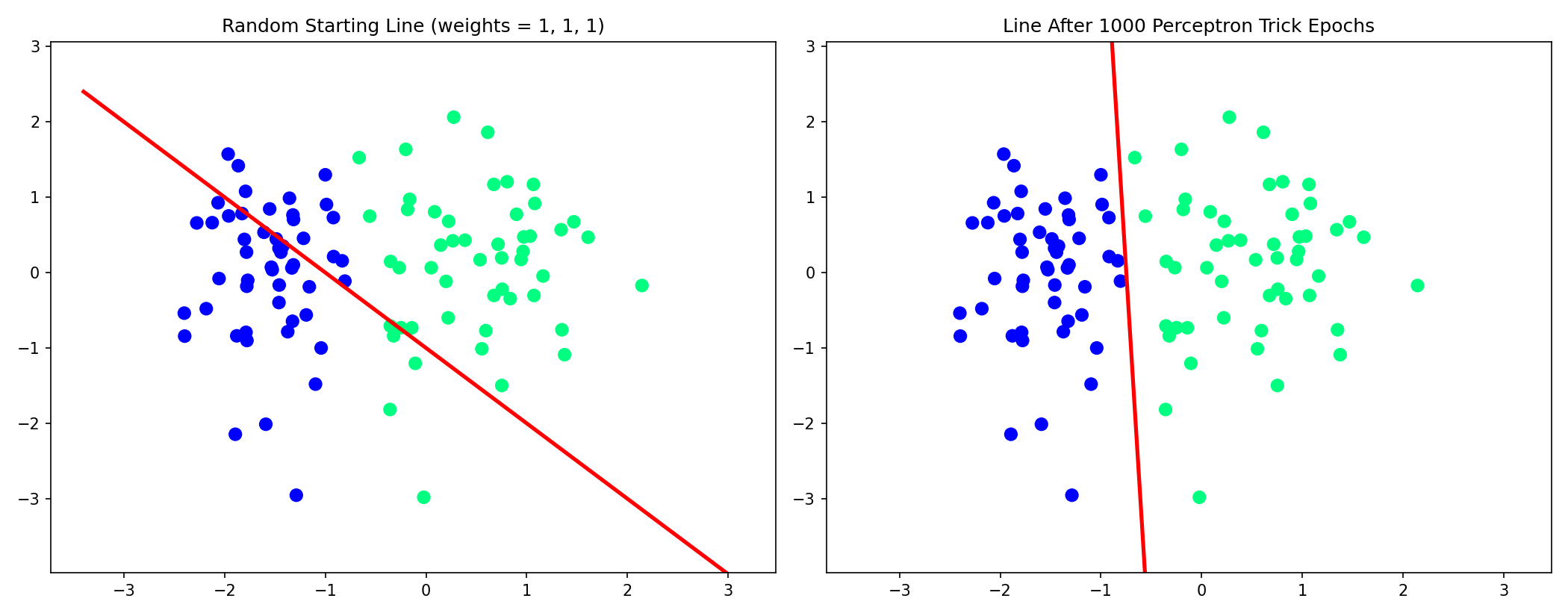
The starting line, from weights = [1, 1, 1], misclassifies 19 of the 100 points. A thousand random nudges later, every point is on the correct side.
9. Watching the Line Move
Recording the line's position every epoch and plotting several snapshots on the same axes shows the rotation happening step by step:
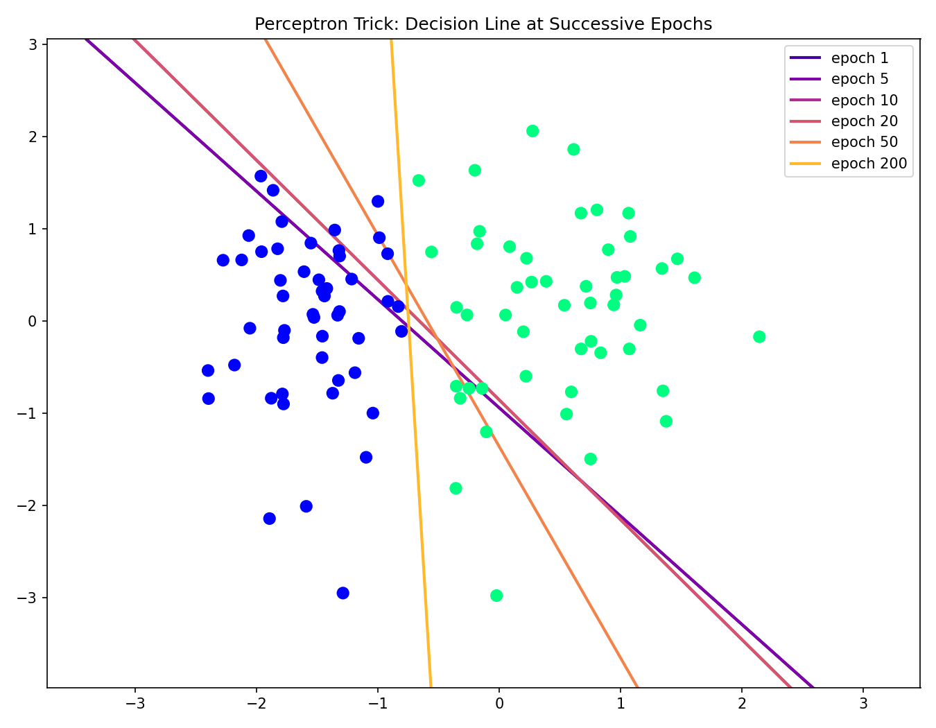
The early epochs barely move the line, most randomly picked points are already correctly classified once the line is roughly in the right neighborhood, so the "do nothing" branch fires most of the time. The visible jumps come from the rarer picks that land on a misclassified point. By epoch 200 the line has rotated most of the way to vertical, sitting almost exactly in the empty gap between the two clusters.
10. What Happens to a Point Exactly on the Line
Section 3 covered three outcomes for : positive, negative, or exactly 0 when a point sits precisely on the boundary. That third case needs a concrete answer once it reaches code, since a prediction has to come out as one class or the other, there's no "undecided" bucket.
The step() function used above settles it by convention:
def step(z):
    return 1 if z > 0 else 0
z > 0 is a strict inequality, so z == 0 falls through to the else and gets predicted as class 0, the negative class. A point sitting exactly on the decision boundary is, by this code's definition, always classified negative, never positive and never left unresolved. That's an arbitrary tie-breaking choice, z >= 0 returning 1 instead would just as validly classify boundary points as positive, but it has to be one or the other, and this is the one the perceptron trick's usual implementation picks.
That choice still feeds back into training the normal way. If a point that's genuinely labeled positive () ever lands exactly on the line (, so by the convention above), the point is a misclassification as far as the update rule is concerned, , not . The line still gets nudged by in the next epoch, even though the point technically wasn't on the wrong side, only balanced precisely on the edge. In practice this case is rare, with real-valued features the odds of landing on exactly 0 are close to zero, and it resolves itself the same way any other misclassified point does: the perceptron trick keeps nudging until nothing (line or point) is left sitting exactly on that boundary in a way the update rule disagrees with.
11. What This Doesn't Guarantee
The Perceptron Trick reliably finds a separating line, but not necessarily the best one. Run it multiple times, or change the random seed, and it converges to a slightly different line each time, anywhere that happens to separate every point counts as success, with no notion of which separating line generalizes best or sits safest in the middle of the gap. Logistic Regression's actual solution, covered from its proper probabilistic foundation in the next post, answers a more specific question and lands on one particular best line rather than merely a working one. The Perceptron Trick's job here was only to build the geometric intuition, weights as a line, misclassification as a nudge, that the real algorithm builds on.