Ch.24: Logistic Regression's Gradient Descent, Derived and Coded

Inspired by: YouTube

Ch.23 derived log loss but ended on the same wall Ridge and Lasso didn't hit: no closed-form solution. Log loss has no algebraic rearrangement that isolates the weights directly, so gradient descent is the only way to minimize it. This post differentiates that loss function with respect to the weight vector, turns the result into a weight-update rule, and codes it from scratch.

1. Setting Up in Matrix Form

Say the dataset has $m$ rows and $n$ feature columns. Stack the rows into a data matrix and prepend a column of all 1s so the intercept can be folded into the same weight vector as every other coefficient:

$X$ is $m \times (n+1)$, $W$ is $(n+1) \times 1$. Every row's prediction, $\hat y_i = \sigma(w_0 + w_1 x_{i1} + \cdots + w_n x_{in})$, is exactly the dot product of that row with $W$, run through sigmoid. Stack all $m$ predictions and the whole thing collapses to one line:

2. Log Loss in Matrix Form

Ch.23's loss function summed a per-row term over all $m$ rows:

Stacking $y_1, \dots, y_m$ into a column vector $y$ and $\hat y_1,\dots,\hat y_m$ into $\hat y$, that sum is a dot product, $y^T\log(\hat y)$ pairs each $y_i$ with its matching $\log(\hat y_i)$ and adds them all up in one shot. So the loss becomes:

Same formula as before, just without the explicit summation sign, the vector notation carries it implicitly.

3. Differentiating With Respect to W

To run gradient descent, $\dfrac{\partial L}{\partial W}$ is needed, a single vector holding $\dfrac{\partial L}{\partial w_0}, \dfrac{\partial L}{\partial w_1}, \dots, \dfrac{\partial L}{\partial w_n}$ all at once. Differentiate the two bracketed terms one at a time.

First term, $y^T\log(\hat y)$. By the chain rule, differentiating $\log(\hat y)$ needs $\dfrac{1}{\hat y}$, then $\hat y = \sigma(XW)$ needs sigmoid's own derivative $\sigma(z)(1-\sigma(z)) = \hat y(1-\hat y)$, then the inner term $XW$ differentiates to $X$. Multiplying the chain together:

The $\hat y$ in the numerator of sigmoid's derivative cancels the $\dfrac{1}{\hat y}$ from the log derivative, leaving just $y(1-\hat y)X$.

Second term, $(1-y)^T\log(1-\hat y)$. Same chain rule, but differentiating $\log(1-\hat y)$ needs $\dfrac{1}{1-\hat y}$ and $(1-\hat y)$ needs $-\hat y(1-\hat y)$ (the negative sign comes along with differentiating the $1-\hat y$ wrapper):

This time the $(1-\hat y)$ terms cancel, leaving $-(1-y)\hat y X$.

Adding the two terms:

The $y\hat y$ terms cancel each other out, leaving a strikingly simple result. Bringing back the $-\dfrac{1}{m}$ from the full loss:

(Written as $X^T(y-\hat y)$ rather than $(y-\hat y)X$ to fix the shapes: $X$ is $m\times(n+1)$ and $(y-\hat y)$ is $m\times1$, so $X^T(y-\hat y)$ multiplies an $(n+1)\times m$ matrix by an $m\times1$ vector, producing the $(n+1)\times1$ vector that matches $W$'s shape.)

4. The Weight Update Rule

Gradient descent subtracts the learning rate times the gradient from the current weights:

The two minus signs cancel, so the update rule is a clean addition: new weights = old weights, plus the learning rate, times the average of $X^T(y-\hat y)$ over all rows. Every weight, $w_0$ through $w_n$, gets updated by this one vector equation simultaneously, no looping over individual coefficients required.

5. Coding It

Translating that directly into NumPy, closely following the source notebook:

def sigmoid(z):
    return 1 / (1 + np.exp(-z))
 
def gd(X, y):
    X = np.insert(X, 0, 1, axis=1)
    weights = np.ones(X.shape[1])
    lr = 0.5
 
    for i in range(5000):
        y_hat = sigmoid(np.dot(X, weights))
        weights = weights + lr * (np.dot((y - y_hat), X) / X.shape[0])
 
    return weights[1:], weights[0]

np.insert(X, 0, 1, axis=1) prepends the all-1s intercept column derived in Section 1. weights starts at all 1s and has shape $(n+1,)$. Inside the loop, y_hat is $\sigma(XW)$ from Section 1, and the update line is Section 4's rule verbatim: np.dot((y - y_hat), X) computes $X^T(y-\hat y)$ (NumPy's 1-D dot between a length-$m$ vector and an $m\times(n+1)$ matrix already produces the $X^T(y-\hat y)$ result, no explicit transpose needed), dividing by X.shape[0] averages over $m$ rows, and lr is $\eta$. weights[0] is the intercept $w_0$, weights[1:] is everything else.

6. Checking It Against scikit-learn

Running this against the same dataset used throughout the Logistic Regression posts and comparing the resulting boundary to sklearn.linear_model.LogisticRegression:

from sklearn.datasets import make_classification
from sklearn.linear_model import LogisticRegression
 
X, y = make_classification(n_samples=100, n_features=2, n_informative=1, n_redundant=0,
                            n_classes=2, n_clusters_per_class=1, random_state=41,
                            hypercube=False, class_sep=20)
 
lor = LogisticRegression(penalty=None, solver="sag")
lor.fit(X, y)
 
coef_, intercept_ = gd(X, y)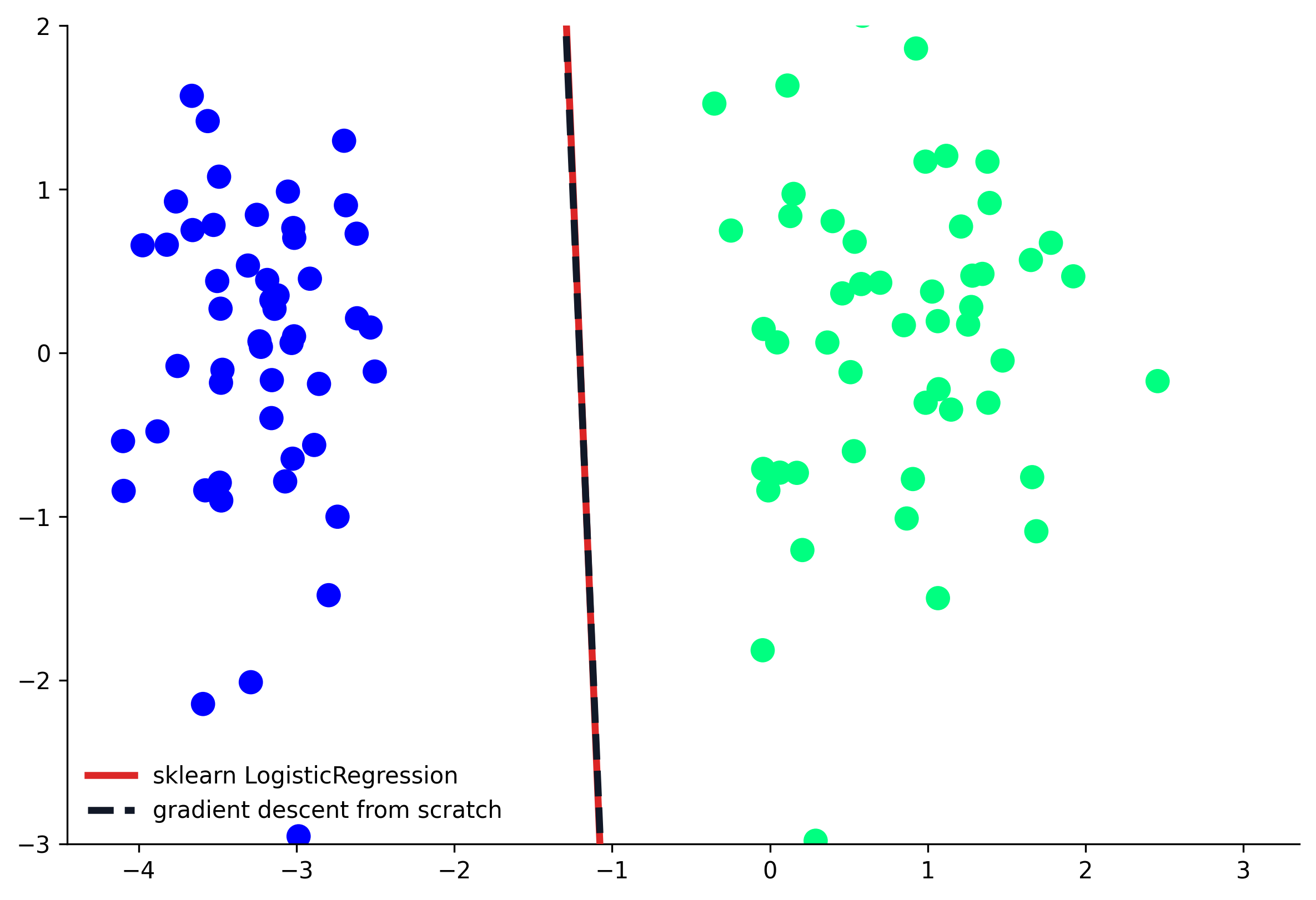

At 5000 epochs and a learning rate of 0.5, the two lines are effectively on top of each other, sklearn finds $w \approx [4.80, 0.20]$, $b \approx 5.78$, and the from-scratch version lands at $w \approx [4.84, 0.21]$, $b \approx 5.83$. That's the direct payoff of deriving the update rule from an actual loss function instead of the ad-hoc push-and-pull rule from Ch.22: the two implementations now agree almost exactly, closing the gap that the sigmoid-perceptron couldn't.

With a much lower epoch count, or a small dataset like this one where a single sharp gap makes convergence sensitive to the exact optimizer, the two lines can still visibly diverge, which is expected: sklearn's sag solver isn't running plain full-batch gradient descent internally, it's a different (and more optimized) iterative method. Full-batch gradient descent over enough epochs converges toward the same optimum, but there's no guarantee the two paths there look identical at every step.

7. Where This Leaves the Series

That closes the arc that started back in Ch.20: starting from the perceptron trick's step function, swapping in sigmoid, deriving log loss from maximum likelihood, and now deriving and coding its gradient descent update rule, a Logistic Regression built entirely from scratch that matches scikit-learn's own implementation. The gd function above runs full-batch (every row, every update); the same loss function supports stochastic and mini-batch variants too, using the same batching ideas from Ch.8 through Ch.10, just applied to this loss instead of squared error.