Ch.31: K-Nearest Neighbors, Intuition and Failure Cases

Inspired by: YouTube

This series moves on from Logistic Regression to a new algorithm: K-Nearest Neighbors (KNN). It's one of the simplest classification algorithms there is, and one of the most intuitive, its entire logic fits in a sentence everyone already understands: you're a lot like the people you spend the most time with.

1. The Core Idea

Motivational speaker Jim Rohn's famous line, "you are the average of the five people you spend the most time with," is a surprisingly exact description of how KNN classifies a point. Given a new, unlabeled point, KNN doesn't build an equation or fit a curve, it just looks at that point's K closest neighbors in the training data and lets them vote. Whatever class most of those neighbors belong to is the predicted class for the new point.

Take the CGPA/IQ/placement dataset used throughout this series' earlier posts. Plot every training student as a point, colored by whether they got placed. Given a new student's CGPA and IQ, KNN answers "will they be placed?" by finding the K most similar students already in the data and going with whichever outcome the majority of them had.

2. The Algorithm, Step by Step

1. Choose K, how many neighbors to consult. Say K=3.
2. Compute the distance from the new (query) point to every point in the training set, usually plain Euclidean distance.
3. Sort those distances and keep the K smallest, the K nearest neighbors.
4. Majority vote: count each neighbor's class label, and assign the query point whichever class got the most votes. It's a small democracy, ask each of the K closest neighbors "what's your class?" and go with the majority answer.

That's the entire algorithm. There's no loss function to minimize and no weights to learn through gradient descent, every part of the computation above happens directly on the raw stored training data.

3. KNN Barely "Trains"

Worth noticing explicitly: everything in Section 2 (computing distances, sorting, voting) happens when a new point needs a prediction, not beforehand. Calling .fit() on a KNN model doesn't compute anything, it just stores the training data for later. All the real work is deferred to prediction time. This makes KNN what's called a lazy learner, and it's the root cause of one of its biggest weaknesses, covered in Section 7.

4. A Real Example

Running KNN on the Breast Cancer Wisconsin dataset (569 patients, 30 numeric measurements per tumor, a binary diagnosis):

from sklearn.model_selection import train_test_split
from sklearn.preprocessing import StandardScaler
from sklearn.neighbors import KNeighborsClassifier
from sklearn.metrics import accuracy_score
 
X_train, X_test, y_train, y_test = train_test_split(X, y, test_size=0.2, random_state=2)
 
scaler = StandardScaler().fit(X_train)
X_train = scaler.transform(X_train)
X_test = scaler.transform(X_test)   # fit on train only, transform test with those same stats
 
knn = KNeighborsClassifier(n_neighbors=5)
knn.fit(X_train, y_train)
 
y_pred = knn.predict(X_test)
print(accuracy_score(y_test, y_pred))

455 training rows, 114 test rows, and KNeighborsClassifier's default K=5 gets 97.4% accuracy. Note the scaler is fit only on the training data and then applied (not re-fit) to the test data, since KNN's entire prediction depends on distance, and distance is unreliable unless every feature is on a comparable scale, a mean area column running into the hundreds would otherwise swamp a mean smoothness column sitting between 0 and 1 in the distance calculation.

5. Choosing K

K is a hyperparameter, and picking it well matters. Two common approaches:

• Heuristic: take $\sqrt{N}$, the square root of the number of training observations, as a rough starting point, rounding to an odd number to avoid tied votes in binary classification. This is a rule of thumb some practitioners reach for, not something rigorously derived.
• Experimental: try a range of K values, evaluate each with cross-validation, and pick whichever performs best.

Sweeping K from 1 to 15 with 10-fold cross-validation on the same dataset:

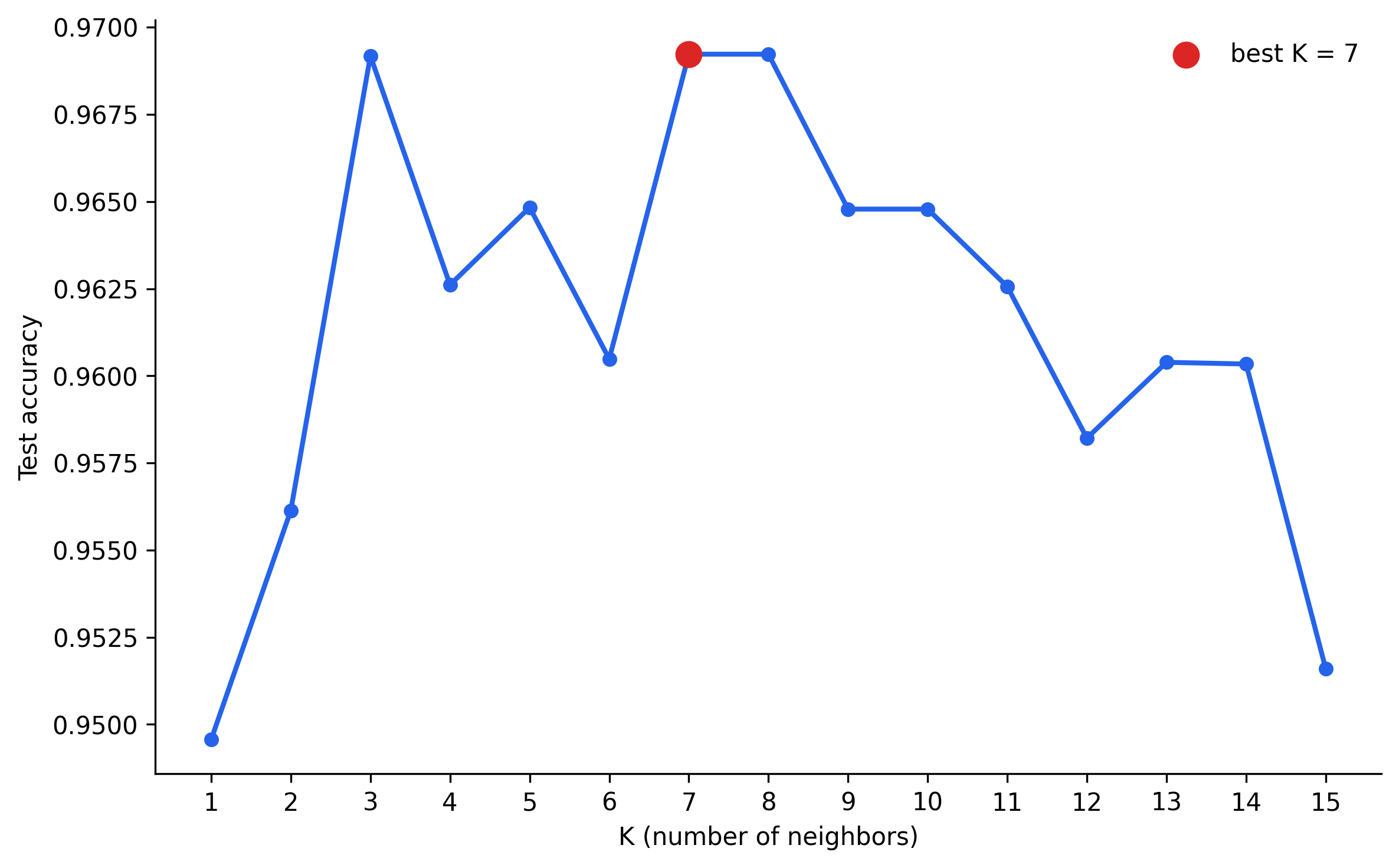
The best cross-validated result here lands at K=7 (accuracy $\approx 0.969$), with a nearby peak at K=3 too, both noticeably ahead of K=1 and the declining tail toward K=15. Exactly the experimental approach: no formula hands over the right K directly, it gets found by trying values and measuring.

6. The Decision Surface

A powerful way to see what any classifier has actually learned, not just KNN, this applies to Logistic Regression, SVMs, Decision Trees, and neural networks too, is to plot its decision surface (also called the decision boundary): color every point in the feature space by what the model would predict there, not just at the training points. Concretely: lay a fine grid of points across the range of the input features, run the trained model's .predict() on every grid point, and color the background by the predicted class. Libraries like mlxtend's plot_decision_regions do this in one function call rather than looping over a grid by hand.

Once that background is colored in, reading off a prediction for any new point is just "which colored region does it fall in?", no separate computation needed, the boundary between regions is the model's decision rule made visible.

7. K Controls Overfitting and Underfitting

Plotting the decision surface at a few different K values on two of the breast cancer features shows exactly how K trades off model complexity:

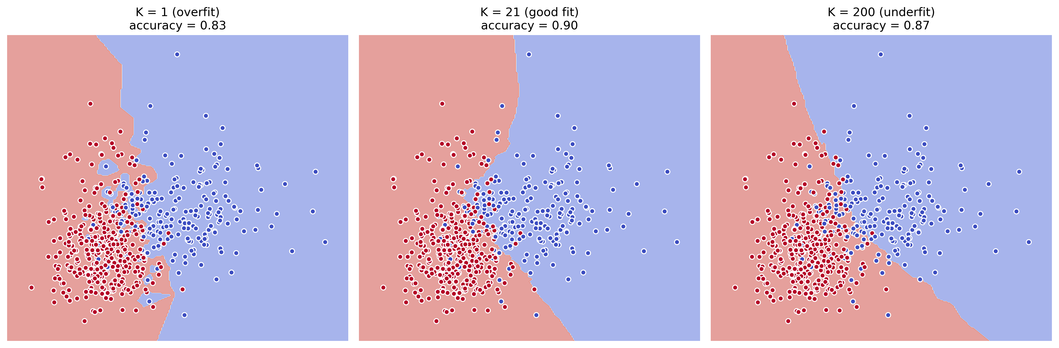
• K=1 (too small): the boundary is jagged and fractured into tiny islands, since every single training point, including outliers and noise, gets to unilaterally carve out its own little region. The model has memorized the training data's every quirk instead of learning its overall shape, textbook overfitting, and it won't generalize well to new points.
• K=200 (too large, out of 455 training rows): the boundary flattens into something close to a single straight cut, because with that many neighbors voting every time, the vote is dominated by whichever class is more common overall, nearly regardless of where the query point actually sits. Taken to its extreme, K equal to the entire training set always predicts the single majority class for every query, completely ignoring the input, textbook underfitting.
• K=21 (in between): the boundary is smooth and follows the data's real shape without chasing individual outlier points, the sweet spot this kind of sweep is meant to find.

Small K overfits, large K underfits, the right value sits in between and gets found experimentally, exactly Section 5's point, now visible directly in the decision surface.

8. Six Situations Where KNN Falls Apart

KNN's simplicity comes with real limitations, worth knowing before reaching for it on a new problem:

1. Large datasets are slow. Because KNN is a lazy learner (Section 3), every single prediction computes distance to every training point, then sorts, then votes. With 500,000 training rows, one prediction means 500,000 distance calculations, unacceptable for a low-latency, real-time application.
2. High-dimensional data breaks distance. With many features, the "curse of dimensionality" makes distance metrics like Euclidean distance increasingly unreliable, points spread out and stop clustering meaningfully. Since KNN relies on distance for literally everything, unreliable distance means unreliable predictions.
3. Outliers distort local regions. Since the prediction near an outlier point is dominated by that single nearby point (worse at low K), a small area around any outlier can get misclassified into the outlier's class, exactly the small-island effect visible at K=1 in Section 7.
4. Unscaled features distort distance. A feature measured in the thousands will dominate a Euclidean distance calculation over a feature measured between 0 and 1, unless every feature is standardized first, Section 4's StandardScaler step is not optional.
5. Imbalanced datasets bias the vote. If 98% of training points belong to one class, most neighborhoods will be dominated by that class regardless of a new point's true label, the same accuracy-distorting effect Ch.25 covered for imbalanced data generally.
6. Poor for inference. KNN can say what class a new point belongs to, but not why, it can't say which feature mattered most in reaching that verdict. It's a solid prediction tool, but a black box when the goal is explaining a decision rather than just making one.

Keeping these six in mind is most of what it takes to use KNN well: it's an excellent, near-zero-assumption baseline on small, clean, well-scaled, balanced, low-dimensional datasets, and a poor choice the moment any of those conditions breaks down.