Ch.22: Swapping the Step Function for Sigmoid

By Ayush Arora•2026-08-27•6 min read

Inspired by: YouTube

Ch.21 ended with a clear gap: the perceptron trick's red line and Logistic Regression's black line both classify every point correctly, but the black line sits with a much wider, safer margin. The perceptron trick's flaw traces back to its algorithm, it only listens to misclassified points and stays completely silent the moment every point is correct. This post fixes that.

1. The Strategy Change

Up to now, the update rule only cared whether a point was misclassified:

Misclassified point → pull the line toward it.
Correctly classified point → do nothing.

The new strategy adds a second behavior for points that are already on the right side:

Misclassified point → pull the line toward it.
Correctly classified point → push the line further away from it.

That single addition means the line never truly stops moving just because every point currently agrees with it. A correctly classified point right near the boundary keeps shoving the line away, which is exactly what widens the margin.

There's a second refinement: how hard a point pulls or pushes should depend on its distance from the line. A misclassified point far from the line is a bigger mistake and should yank harder than one that's barely on the wrong side. A correctly classified point close to the line is at risk of being wrong soon, so it should push harder than one already comfortably far away.

2. Why the Step Function Can't Do This

The old update rule was:

W_{new} = W_{old} + \eta(y - \hat y)x

With step, $\hat y$ is always exactly 0 or 1. Whenever a point is correctly classified, $y - \hat y$ collapses to exactly 0, and the entire update term vanishes, no matter how close that point sits to the line. The step function can't express "correctly classified, but only just" versus "correctly classified with room to spare", it only has two possible outputs.

To get graded pushes and pulls, $\hat y$ needs to become a continuous number instead of a hard 0 or 1. That's what the sigmoid function is for:

\sigma(z) = \frac{1}{1 + e^{-z}}

Sigmoid takes any real number and squashes it into the range (0, 1), approaching 1 for large positive inputs, approaching 0 for large negative inputs, and landing exactly at 0.5 when the input is 0, i.e. exactly on the line. That last property lines up with distance-from-the-line: a point far on the positive side gets a $\hat y$ close to 1, a point far on the negative side gets a $\hat y$ close to 0, and points near the boundary get $\hat y$ near 0.5. So $y - \hat y$ is now a graded number that's never exactly 0 unless a point is infinitely far from the line, which means every single point, correctly classified or not, contributes something to every update.

3. Implementing It

The only change from Ch.21's code is which function computes y_hat:

def sigmoid(z):
    return 1 / (1 + np.exp(-z))
 
def perceptron(X, y, epochs=1000, lr=0.1):
    X = np.insert(X, 0, 1, axis=1)
    weights = np.ones(X.shape[1])
 
    for i in range(epochs):
        j = np.random.randint(0, 100)
        y_hat = sigmoid(np.dot(X[j], weights))
        weights = weights + lr * (y[j] - y_hat) * X[j]
 
    return weights[0], weights[1:]

step(z) becomes sigmoid(z), and nothing else about the loop changes. The update rule $W \mathrel{+}= \eta(y-\hat y)X$ is untouched, it's just operating on a continuous $\hat y$ now instead of a binary one.

4. Reading the Four Cases Through Sigmoid

The same four combinations of true label and prediction from Ch.20 still apply, but they now behave differently:

Correctly classified positive ( $y=1$ , point far on the positive side): $\hat y$ is close to 1, so $y - \hat y$ is small but not zero. The update still nudges the line, just gently, pushing it slightly further away from this point.
Correctly classified negative ( $y=0$ , point far on the negative side): $\hat y$ is close to 0, so $y - \hat y$ is again small but nonzero, gently pushing the line away on that side too.
Misclassified positive ( $y=1$ , but the point sits on the negative side): $\hat y$ is closer to 0 here, so $y - \hat y$ is large, and the line gets pulled strongly toward this point.
Misclassified negative ( $y=0$ , but the point sits on the positive side): $\hat y$ is closer to 1, so $y - \hat y$ is large and negative, again pulling the line strongly, this time in the other direction.

And distance still matters within each case: a correctly classified point sitting right next to the line has $\hat y$ close to 0.5 rather than close to 0 or 1, so $y - \hat y$ is bigger for it than for a point far away on the correct side, meaning nearby correct points push harder than distant correct ones. Exactly the graded behavior the step function couldn't give.

5. Comparing All Three Lines

Running the sigmoid version on the same dataset as Ch.21 and plotting it alongside the original step-function perceptron and Scikit-Learn's LogisticRegression:

from sklearn.linear_model import LogisticRegression
 
intercept_step, coef_step = perceptron(X, y)   # step version, from Ch.21
intercept_sig, coef_sig = perceptron(X, y)      # sigmoid version, this post
 
lor = LogisticRegression()
lor.fit(X, y)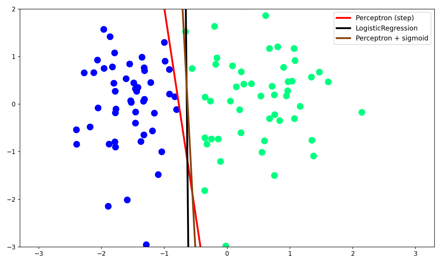

Scatter plot of two linearly separable clusters, blue on the left and green on the right. Three lines cross the gap between them: a red line (step-function perceptron) sitting furthest from LogisticRegression's black line, a brown line (sigmoid perceptron) sitting much closer to black, and the black line itself. Brown and black nearly overlap but are still visibly distinct

The brown sigmoid line sits dramatically closer to the black Logistic Regression line than the red step-function line did. Swapping in sigmoid was the right move in the right direction, every point now contributes to every update, and the line keeps improving its margin even after every point is technically correct.

But look closely: brown and black still aren't the same line. The gap has shrunk a lot, but it hasn't closed completely. Something is still missing.

6. What's Still Missing

The video ends on this open question deliberately: sigmoid fixed the "correctly classified points do nothing" problem, but the sigmoid-perceptron still isn't identical to real Logistic Regression. The remaining gap comes from how the update rule was changed, it was changed by intuition and analogy ("make correct points push, make it graded by distance"), not derived from an actual objective function that defines what "best line" precisely means.

Real Logistic Regression doesn't patch the perceptron trick's update rule by hand. It starts from a loss function built on these same sigmoid probabilities, and derives its update rule mathematically by minimizing that loss. That's the next step: writing down what makes a line "good" as an actual number to minimize, rather than a set of ad-hoc push-and-pull rules, which is exactly what closes this final gap between brown and black.

View all chapters in Machine Learning Algorithms →