
Ch.8: Batch Gradient Descent for Multiple Linear Regression
Inspired by: YouTube
Ch.1 through Ch.6 built up the theory and closed-form OLS solution for both simple and multiple linear regression. Ch.7 introduced Gradient Descent, derived partial derivatives for the single-feature case (), and showed that the update loop converges to the same solution as OLS on synthetic data.
In this post, we extend that same logic to the multi-feature case: input columns, parameters to learn simultaneously. We will derive why the coefficient update becomes a dot product with , implement a GDRegressor class that handles any number of features without changing a single line of the loop body, and benchmark it on sklearn's diabetes dataset against closed-form OLS.
From One Feature to Many: The Setup
In the previous post, the model had one slope and one intercept . Every real dataset has more features. The diabetes dataset, for example, has 10 clinical measurements per patient. The general multiple linear regression model is:
where is the intercept and are the slope coefficients. For a dataset with input columns, you have parameters to estimate.
To apply gradient descent, you need partial derivatives of the loss with respect to each one. With 10 features that is 11 separate update equations, and with 1,000 features it is 1,001. Writing them out individually does not scale. The solution is to derive a single vectorized update rule that handles all coefficients in one matrix operation.
Deriving the Vectorized Update Rule
Prediction as a Single Matrix Product
Rather than singling out the intercept, build on the augmented-matrix trick from Ch.6 directly: prepend a column of 1s to , so every row picks up an extra entry , and stack every parameter, intercept included, into one vector of length . The entire prediction for every row is then one matrix product:
Written out with the augmented column explicit:
There is no separate scalar equation for , it's just row 0 of , paired with that leading column of 1s.
Loss Function
We use Mean Squared Error (MSE) loss averaged over all training rows, written the same way Ch.6 writes SSE, just scaled by :
Whether you use MSE or SSE (sum, not mean) does not change which minimizes the loss, only the scale of the gradient. We use MSE here to keep gradient magnitudes independent of dataset size.
Differentiating the Matrix Loss
Ch.6 already worked out term by term. The only difference here is the extra from using MSE instead of SSE, which carries straight through:
This single expression is the gradient for every parameter at once, intercept included, no separate cases needed. The update rule at each epoch is:
In code, np.dot(X_train.T, residuals) (or equivalently residuals @ X_train when residuals is a 1D array, using NumPy's broadcasting) gives a vector of length , one gradient per coefficient including the intercept. This replaces scalar equations with a single line of NumPy, and the loop body doesn't grow as grows.
Why the code below still splits
intercept_out separately: Mathematically is just row 0 of . But NumPy code doesn't need to physically prepend a 1s column to get that benefit: is justnp.mean(residuals), so the intercept update can be computed directly without ever materializing the extra column. TheGDRegressorclass below does exactly that, one line for the intercept, one matrix operation for the rest, algebraically identical to running the single augmented update above and splitting the result back into and .
Implementing GDRegressor from Scratch
The implementation below follows the source notebook batch-gradient-descent.ipynb exactly.
Loading the Diabetes Dataset
from sklearn.datasets import load_diabetes
import numpy as np
from sklearn.linear_model import LinearRegression
from sklearn.metrics import r2_score
from sklearn.model_selection import train_test_split

X, y = load_diabetes(return_X_y=True)
print(X.shape)  # (442, 10)
print(y.shape)  # (442,)
The dataset has 442 patients, each described by 10 standardized clinical features (age, sex, BMI, blood pressure, and six serum measurements). The target is a quantitative measure of diabetes progression one year after baseline. Crucially, sklearn's load_diabetes already returns normalized features, so no additional scaling step is needed here.
X_train, X_test, y_train, y_test = train_test_split(
    X, y, test_size=0.2, random_state=2
)
print(X_train.shape)  # (353, 10)
Benchmarking with sklearn's LinearRegression
Before building our own optimizer, we establish the OLS ceiling:
reg = LinearRegression()
reg.fit(X_train, y_train)

y_pred = reg.predict(X_test)
print("OLS intercept:", reg.intercept_)
# 151.88331005254165

print("OLS coef_:", reg.coef_)
# [ -9.16, -205.46,  516.69,  340.62, -895.55,
#   561.22,  153.89,  126.73,  861.13,   52.42]

print("OLS R2:", r2_score(y_test, y_pred))
# 0.4399
The OLS model explains about 44% of the variance in test disease progression scores. This is our target to approach.
The GDRegressor Class
class GDRegressor:
    def __init__(self, learning_rate=0.5, epochs=1000):
        self.lr = learning_rate
        self.epochs = epochs
        self.coef_ = None
        self.intercept_ = None

    def fit(self, X_train, y_train):
        # Initialize: intercept to 0, all coefficients to 1
        self.intercept_ = 0
        self.coef_ = np.ones(X_train.shape[1])

        for _ in range(self.epochs):
            # Forward pass: compute predictions
            y_hat = X_train @ self.coef_ + self.intercept_

            # Intercept gradient: -2 * mean(residuals)
            intercept_der = -2 * np.mean(y_train - y_hat)
            self.intercept_ -= self.lr * intercept_der

            # Coefficient gradient: -2/n * X_train.T @ residuals
            coef_der = -2 * np.dot((y_train - y_hat), X_train) / X_train.shape[0]
            self.coef_ -= self.lr * coef_der

    def predict(self, X):
        return X @ self.coef_ + self.intercept_
A few design details worth noting:
Initialization strategy. The intercept starts at zero because it is a single scalar and zero is a neutral starting point. The coefficients are initialized to ones (np.ones(X_train.shape[1])), which avoids the symmetry-breaking problem of all-zeros initialization while remaining simple. The number of coefficients is inferred from X_train.shape[1] at fit time, so the class works for any number of features without modification.
np.dot((y_train - y_hat), X_train) computes the dot product of a 1D residual array (shape (n,)) with a 2D matrix (shape (n, k)), yielding a 1D result of shape (k,). NumPy lines up the residual array against the matrix's first axis (the rows) and sums over that axis for each of the columns independently, which is exactly the "multiply residuals by one feature column and sum" computation from the derivation above, done for all columns at once. This is equivalent to X_train.T @ residuals (transpose to shape , then matrix-multiply by the residual vector), but skips the explicit transpose.
Simultaneous update. Both intercept_der and coef_der are computed from the same y_hat at the start of the epoch, before either parameter is modified. This is important: if you updated the intercept first and then recomputed y_hat to get the coefficient gradient, the two updates would be using different parameter states, which is not the standard gradient descent algorithm.
Running and Evaluating
gd = GDRegressor(learning_rate=0.5, epochs=1000)
gd.fit(X_train, y_train)

print("GD intercept:", gd.intercept_)
# 152.01352

print("GD coef_:", gd.coef_)
# [ 14.39, -173.73,  491.55,  323.92, -39.33,
#  -116.01, -194.04,  103.38,  451.63,   97.57]

y_pred_gd = gd.predict(X_test)
print("GD R2:", r2_score(y_test, y_pred_gd))
# 0.4535
The custom GDRegressor achieves R² = 0.4535 on the test set, slightly above the OLS benchmark of 0.4399. The intercept converges to 152.01, close to OLS's 151.88. Most coefficients agree in sign and rough magnitude (negative , large positive and ), but three flip sign entirely: , , and . (age) is near zero in both models, so its flip is noise around a coefficient that barely matters. (s2) and (s3) are each strongly correlated with a third feature, (s4), with and respectively. That shared correlation flattens the loss surface along the directions those coefficients control: many different combinations produce nearly the same predictions, so the exact split OLS computes and the split 1000 epochs of gradient descent has reached can differ substantially, even in sign, without the R² score moving much. With more epochs or a finer learning rate sweep, the two solutions would align more closely.
Convergence Behavior
The chart below shows the training MSE and R² over the 1000 epochs, generated by running the exact GDRegressor loop above:
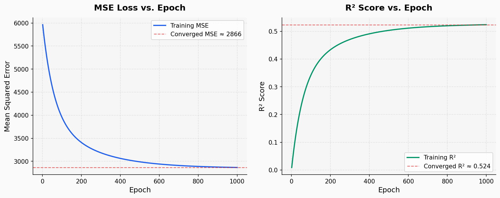
The convergence pattern is characteristic of batch gradient descent on a convex loss surface: the largest gains happen in the first 200 epochs as the parameters escape from their poor initialization (all coefficients at 1). After epoch 400 the curves flatten noticeably, and by epoch 800 improvement per epoch is marginal. The final training R² lands near 0.524, higher than the test R² of 0.454, which is normal: the training set is what the optimizer directly minimizes.
An important note on the convergence rate here: the diabetes features are already normalized (zero mean, unit variance per feature), which is why a learning rate as high as 0.5 is stable. On raw unscaled data, that same learning rate would cause the coefficients for high-variance features to diverge.
Coefficient Comparison
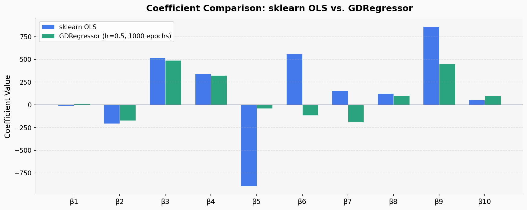
Seven of the ten coefficients agree in sign; , , and flip. is near zero in both models (OLS: , GD: ), so the flip is noise around a coefficient that barely matters. and are more interesting: OLS puts them at and , while GD lands at and . Both are strongly correlated with ( and ), which flattens the loss surface along their joint directions, so OLS's exact split between the three correlated coefficients and gradient descent's 1000-epoch approximation of that split can disagree substantially, even in sign. The magnitude divergence is largest for (OLS: , GD: ) and (OLS: , GD: ), features with the steepest loss curvature, meaning gradient descent has the most work to do along those axes. More epochs would close both gaps. The test R² gap is small (0.44 vs 0.45) because these large, partially-compensating coefficients affect individual predictions less than their raw magnitudes suggest.
What Makes This "Batch" Gradient Descent
The word "batch" in "Batch Gradient Descent" refers to the fact that every single epoch processes all training rows before taking one parameter update step.
In the fit loop above, y_hat = X_train @ self.coef_ + self.intercept_ computes predictions for all 353 training rows at once. The gradient coef_der is averaged over all 353 residuals. Only then do the parameters move. This is the defining characteristic of batch gradient descent: one gradient computation per epoch, using the full dataset.
The alternative approaches, Stochastic Gradient Descent (SGD) and Mini-Batch Gradient Descent, change precisely this one aspect: how many rows are used per gradient estimate and update step. The mathematical form of the update rule, the chain rule derivation, and the parameter initialization are all identical. The entire difference is in the loop body:
| Variant | Rows used per update | Updates per epoch |
|---|---|---|
| Batch GD (this post) | All rows | 1 |
| Stochastic GD | 1 row | |
| Mini-Batch GD | rows (batch size) |
For the diabetes dataset with training rows, batch GD takes 1 update per epoch. Stochastic GD would take 353 updates per epoch, one per row. Mini-Batch GD with batch size 32 would take about 11 updates per epoch.
The practical implication: batch GD is the safest choice when the dataset fits in memory and the loss surface is convex (guaranteed for linear regression's squared error). When the dataset is large or the loss is non-convex, SGD or mini-batch GD become preferable because they provide noisier but more frequent gradient signals.
Summary & Key Takeaways
- Extending to features: Multiple linear regression requires parameters ( slopes plus one intercept). Gradient descent applies the same chain rule to each, producing update equations per epoch.
- The intercept isn't special: with a column of 1s prepended to (the Ch.6 augmented-matrix trick), is just the general update with plugged in, not a separately derived rule.
- Vectorized update for all parameters: . The matrix transpose turns the per-residual, per-column products into a single dot product that yields all gradients simultaneously, intercept included.
- Why transposing works: produces a -dimensional vector where entry is , exactly the sum needed for . The transpose swaps rows and columns so each feature's (and the intercept's constant "feature") values end up in a row, enabling a single matrix-vector multiply.
- Initialization: Intercept to 0, coefficients to ones. The shape of the coefficient array is inferred from
X_train.shape[1]at fit time, making the class feature-count agnostic. - Simultaneous update: Both gradients are computed from the same
y_hatbefore either parameter is updated. Updating intercept first and recomputingy_hatmid-epoch would violate the standard gradient descent algorithm. - Batch GD result on diabetes: With
learning_rate=0.5andepochs=1000, the customGDRegressorachieves test R² = 0.4535, modestly above OLS's 0.4399. Seven of ten coefficients agree in sign; the three that flip include a near-zero coefficient and two strongly collinear features whose individual OLS values are unstable. More epochs would close the remaining magnitude gap. - What "batch" means: Every epoch consumes all training rows before taking one gradient step. This is the defining property that distinguishes batch GD from its faster, noisier variants.
In the next post, we explore Stochastic Gradient Descent (updating parameters after every single training row) and Mini-Batch Gradient Descent (updating after each small batch of rows), examining how each variant trades gradient accuracy for computational efficiency on large datasets.