Ch.10: Mini-Batch Gradient Descent

By Ayush Arora•2026-08-16•12 min read

Inspired by: YouTube

We now have two gradient descent variants that sit at opposite extremes. Batch GD (Ch.8) looks at every row before making a single update: smooth and stable, but slow and impossible to run on data too big for RAM. SGD (Ch.9) looks at just one random row per update: fast to get moving and cheap on memory, but its path is so noisy it never settles down. Mini-batch gradient descent is the obvious question you'd ask after seeing both: what if, instead of "all rows" or "one row," you updated on a small random handful of rows at a time?

That is the entire idea. Everything else in this post is working out the consequences.

The Idea in One Picture

Think of the three variants as answering the same question differently: "How many rows do I look at before I update the parameters?"

Variant	Rows per update	Updates per epoch (n = 353 rows)
Batch GD	all $n$	1
SGD	1	$n$ = 353
Mini-Batch GD	a batch of size $b$	$n / b$

Pick $b = n$ and mini-batch GD becomes batch GD. Pick $b = 1$ and it becomes SGD. Everything in between is mini-batch GD. It is not a third algorithm bolted onto the first two; it is the general case that the other two are special cases of.

Why would a batch of, say, 7 rows out of 353 be better than either extreme?

Faster than batch GD, because you don't wait to see all 353 rows before the parameters move even once. You get many small updates per epoch instead of one big one.
Smoother than SGD, because averaging the gradient over 7 rows cancels out some of the randomness that a single row carries. One noisy row can point in a weird direction; seven rows averaged together are less likely to.
Fast to compute, because unlike SGD's row-by-row Python loop, a batch of 7 rows can still be handled with a single vectorized NumPy matrix operation (X_train[idx] @ coef_), just like batch GD does for the full dataset.

Mini-batch GD is not a compromise that gives up the best of both; in practice it keeps most of what makes each extreme good.

The Math: Same Derivative, Different Group Size

Recall the two derivatives we already derived:

Batch GD (average over all $n$ rows):

$\frac{\partial L}{\partial \beta_j} = -\frac{2}{n} \sum_{i=1}^n (y_i - \hat{y}_i) \cdot x_{ij}$

SGD (a single row $i$ , no averaging):

$\frac{\partial L}{\partial \beta_j} = -2 (y_i - \hat{y}_i) \cdot x_{ij}$

Mini-batch GD just changes what you sum over. Instead of "all $n$ rows" or "one row," you sum over a randomly chosen batch $B$ of size $b$ , and average by $b$ instead of $n$ :

$\frac{\partial L}{\partial \beta_j} = -\frac{2}{b} \sum_{i \in B} (y_i - \hat{y}_i) \cdot x_{ij}$

Set $b = n$ (the batch is the whole dataset) and this collapses exactly to the batch GD formula. Set $b = 1$ (the batch is one row, and averaging one number by 1 does nothing) and it collapses exactly to the SGD formula. There is no new math here, just a different-sized group inside the sum.

Implementing `MBGDRegressor` from Scratch

The implementation follows the source notebook in day52-types-of-gradient-descent, the same folder as Ch.9's SGD implementation. Same dataset, same split, same class shape.

The Dataset (Same as Ch.8 and Ch.9)

from sklearn.datasets import load_diabetes
import numpy as np
import random
from sklearn.linear_model import LinearRegression
from sklearn.metrics import r2_score
from sklearn.model_selection import train_test_split
 
X, y = load_diabetes(return_X_y=True)
X_train, X_test, y_train, y_test = train_test_split(
    X, y, test_size=0.2, random_state=2
)
print(X_train.shape)  # (353, 10)

The `MBGDRegressor` Class

class MBGDRegressor:
    def __init__(self, batch_size, learning_rate=0.01, epochs=100):
        self.coef_ = None
        self.intercept_ = None
        self.lr = learning_rate
        self.epochs = epochs
        self.batch_size = batch_size
 
    def fit(self, X_train, y_train):
        # Initialize exactly like GDRegressor and SGDRegressor
        self.intercept_ = 0
        self.coef_ = np.ones(X_train.shape[1])
 
        for i in range(self.epochs):
            for j in range(int(X_train.shape[0] / self.batch_size)):
                # Pick `batch_size` random row indices, no repeats within a batch
                idx = random.sample(range(X_train.shape[0]), self.batch_size)
 
                # Vectorized prediction for the whole batch at once
                y_hat = np.dot(X_train[idx], self.coef_) + self.intercept_
 
                # Intercept gradient: mean residual over the batch
                intercept_der = -2 * np.mean(y_train[idx] - y_hat)
                self.intercept_ -= self.lr * intercept_der
 
                # Coefficient gradient: dot product over the batch (this is the sum, not yet divided by b)
                coef_der = -2 * np.dot((y_train[idx] - y_hat), X_train[idx])
                self.coef_ -= self.lr * coef_der
 
    def predict(self, X_test):
        return np.dot(X_test, self.coef_) + self.intercept_

Walk through what changed compared to SGDRegressor from Ch.9:

The inner loop runs X_train.shape[0] // batch_size times per epoch, not X_train.shape[0] times. If you pick batch_size = 7 on 353 rows, the inner loop runs 50 times per epoch, not 353 times. Each of those 50 iterations touches 7 rows, for roughly $50 \times 7 = 350$ rows seen per epoch, close to the full dataset (some rows get skipped or repeated across batches because sampling is random each time, not a clean partition).

random.sample(range(n), batch_size) picks batch_size distinct indices without replacement, unlike SGD's np.random.randint, which could pick the same row twice in a row. Within one batch you always get batch_size different rows. Across batches, though, there's no bookkeeping to guarantee every row gets visited exactly once per epoch. This is a real design looseness in mini-batch GD compared to a "proper" epoch that shuffles once and slices cleanly, but it's how the reference implementation does it, and it works fine in practice.

np.dot(X_train[idx], self.coef_) now operates on a matrix of shape (batch_size, 10), not a single row. This is a real (if tiny) matrix multiply, so y_hat comes out as a (batch_size,) vector of predictions, one per row in the batch. Compare this to SGD, where y_hat was a bare scalar.

The intercept gradient uses np.mean(...) over the batch, exactly like batch GD's np.mean over the full dataset, just averaging over 7 rows instead of 353. The coefficient gradient uses np.dot(residuals, X_train[idx]), which sums (not averages) the product of each row's residual with its features. That sum, divided by batch_size, would be the textbook mean-gradient formula. The code above skips the explicit division and folds that scaling into the learning rate instead; the learning rate of 0.01 was picked to make it converge well specifically because of this. If you compare it against a hand-derived formula and the constant looks "off" by a factor of batch_size, this is why.

Running and Evaluating

mbr = MBGDRegressor(batch_size=int(X_train.shape[0] / 50), learning_rate=0.01, epochs=100)
mbr.fit(X_train, y_train)
# batch_size = 353 // 50 = 7
 
print("MBGD intercept:", mbr.intercept_)
# 151.10
 
print("MBGD coef:", mbr.coef_)
# [  30.4, -138.9,  449.7,  303.0,  -19.6,
#    -93.8, -190.7,  113.0,  419.3,  110.0]
 
y_pred_mbgd = mbr.predict(X_test)
print("MBGD R2:", r2_score(y_test, y_pred_mbgd))
# 0.4516

The batch size here (7 rows out of 353) is not derived from theory; it's chosen so the dataset splits into roughly 50 batches per epoch (353 // 50 = 7). This "how many batches do I want per epoch" framing is a common and reasonable way to pick batch_size in practice: it's easier to reason about "50 updates per epoch" than to guess a raw row count.

At 100 epochs, here's how all four approaches compare on test R²:

Model	Epochs	Test R²
sklearn OLS (Ch.8)	closed-form	0.4399
Batch GDRegressor	100	0.3202
SGDRegressor	100	0.4480
MBGDRegressor	100	0.4516

At only 100 epochs, batch GD hasn't caught up yet (it needed 1000 epochs in Ch.8 to reach 0.4535). Both SGD and mini-batch GD are already ahead of OLS at 100 epochs, and mini-batch GD edges out SGD slightly here. This is the epoch-efficiency advantage in action: more updates per epoch means faster progress in wall-clock epoch count, regardless of whether those updates come one row at a time or seven rows at a time.

Why Mini-Batch Converges as Fast as SGD, but Smoother

The chart below trains all three variants for 100 epochs on the same data and tracks training R² after every epoch.

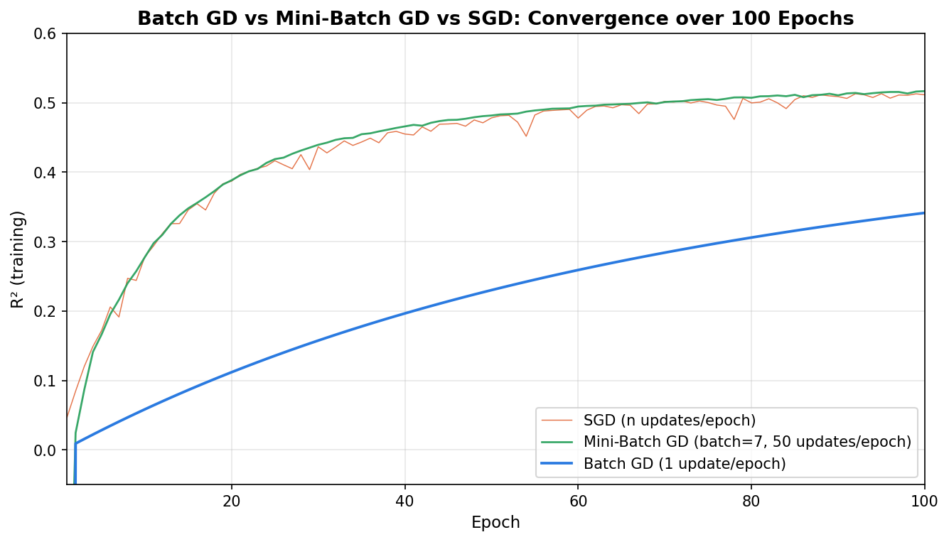
Line chart comparing training R² per epoch for Batch GD, Mini-Batch GD, and SGD over 100 epochs. SGD (thin orange line) and Mini-Batch GD (thick green line) both rise quickly and track each other closely, reaching about 0.51-0.52 by epoch 100, with SGD visibly jagged and Mini-Batch GD much smoother. Batch GD (thick blue line) rises far more slowly, reaching only about 0.34 by epoch 100.

Three things to notice:

SGD (orange) and mini-batch GD (green) rise at almost the same rate, both crossing R² = 0.4 by around epoch 20, while batch GD (blue) is still below 0.15 at that point. This is the direct consequence of update count: SGD gets 353 updates per epoch, mini-batch GD gets 50, batch GD gets 1. More updates per epoch means faster progress per epoch, almost regardless of how noisy each individual update is.

The green line is visibly smoother than the orange one. Zoom into any stretch, say epochs 40 to 60, and SGD's line jitters up and down noticeably while mini-batch GD's line is a steady, gently climbing curve. This is exactly the averaging effect from the math above: each mini-batch update averages the gradient over 7 rows, and outlier rows get diluted by the other 6 rows in the batch instead of swinging the parameters on their own.

Batch GD is not "wrong," it's just slow in epoch count. Given enough epochs (Ch.8 used 1000), batch GD would eventually reach the same R² and settle there permanently, with zero oscillation, because it uses the exact full-dataset gradient every time. At 100 epochs, it simply hasn't had enough updates yet: 100 updates total, versus mini-batch GD's 5,000 and SGD's 35,300.

This is the practical case for mini-batch GD: you get SGD's speed of early progress without SGD's amount of noise once you get close to the optimum.

Choosing the Batch Size

batch_size is the one new hyperparameter mini-batch GD introduces, and it directly controls where you sit on the batch-GD-to-SGD spectrum:

Small batch (close to 1): behaves more like SGD. Fast per-epoch progress, more noise, cheaper per-update memory footprint.
Large batch (close to $n$ ): behaves more like batch GD. Smoother convergence, but slower per-epoch progress and a bigger memory footprint per update.
Common practical choices: powers of 2 like 32, 64, 128, or 256, mostly because that plays well with how GPUs and vectorized libraries lay out memory. In this post, the batch size was picked from "how many batches per epoch do I want" (50), which is a perfectly reasonable alternative framing when you're reasoning about a small dataset rather than tuning for hardware.

There's no formula that tells you the "correct" batch size in advance; it's a hyperparameter you tune like the learning rate, usually by trying a few values and comparing validation performance and convergence smoothness.

Mini-Batch GD in Practice: `SGDRegressor.partial_fit`

Scikit-learn doesn't ship a separate MiniBatchGDRegressor class. Instead, you get mini-batch behavior out of SGDRegressor by feeding it batches manually through partial_fit, which the source notebook demonstrates:

from sklearn.linear_model import SGDRegressor
 
sgd = SGDRegressor(learning_rate='constant', eta0=0.1)
 
batch_size = 35
for i in range(100):
    idx = random.sample(range(X_train.shape[0]), batch_size)
    sgd.partial_fit(X_train[idx], y_train[idx])
 
y_pred = sgd.predict(X_test)
print("R2:", r2_score(y_test, y_pred))
# 0.4112

partial_fit is the key method here: unlike .fit(), which resets the model and trains from scratch on whatever data you pass it, partial_fit updates the existing parameters using only the batch you hand it, then keeps them for the next call. Calling it 100 times with a fresh random batch of 35 rows each time is functionally mini-batch gradient descent, just with sklearn's optimized internals doing the update instead of our hand-written NumPy.

This pattern is also how you'd handle a dataset that doesn't fit in memory at all: read one batch off disk, partial_fit on it, discard it, read the next batch. Neither .fit() on the full X_train nor our from-scratch classes could do this, since both assume the whole array is already in RAM. partial_fit is the sklearn feature that makes true out-of-core training possible.

Summary & Key Takeaways

Mini-batch GD is the general case: batch GD ( $b = n$ ) and SGD ( $b = 1$ ) are its two endpoints, not separate algorithms. The gradient formula only changes in what group of rows you average over.
The implementation reuses everything: MBGDRegressor differs from SGDRegressor only in how many rows the inner loop samples (random.sample for batch_size rows, instead of one randint draw) and that the prediction/gradient math is now a small vectorized batch operation instead of a scalar one.
More updates per epoch than batch GD, fewer Python-loop iterations than SGD: with $b = 7$ on 353 rows, you get 50 updates per epoch, each one a fast vectorized NumPy call over 7 rows, not 353 individual scalar updates.
Convergence speed close to SGD, smoothness close to batch GD: averaging the gradient over a small batch cancels out some of the single-row noise that makes SGD's path so jagged, while still getting far more updates per epoch than batch GD.
batch_size is a new tunable hyperparameter: small batches behave more like SGD, large batches behave more like batch GD, and there's no universally correct value; it's chosen empirically or by hardware convenience (powers of 2).
No dedicated sklearn class: mini-batch behavior comes from repeatedly calling SGDRegressor.partial_fit() on random batches rather than calling .fit() once. This same pattern (partial_fit on successive chunks) is also how you'd train on a dataset too large to fit in memory.

Across these three posts, the pattern to remember is: the trade-off is always speed of convergence in epoch count versus smoothness of the path to the optimum, and batch size is the dial that lets you choose where on that spectrum you want to sit.

View all chapters in Machine Learning Algorithms →