Ch.14: Ridge Regression: The Math and the Code

Inspired by: YouTube

In the previous post, we established why Ridge Regression works: appending a penalty term $\lambda m^2$ to the OLS loss function makes large, unstable coefficients expensive, which pulls the fitted line away from a perfect but brittle fit on the training set and toward one that generalizes better.

This post picks up where that one left off. We derive the closed-form formula that actually produces the shrunk coefficient, first for the single-feature case, then for the general n-dimensional case using matrix calculus, and implement both from scratch to confirm they land on exactly the coefficients Scikit-Learn's Ridge class does.

1. Deriving the Closed-Form Solution for One Feature

Recall simple linear regression's loss with the L2 penalty added:

$L = \sum_{i=1}^n (y_i - mx_i - b)^2 + \lambda m^2$

To minimize $L$, take partial derivatives with respect to $b$ and $m$ and set both to zero.

Differentiating with respect to $b$:

$\frac{\partial L}{\partial b} = \sum_{i=1}^n 2(y_i - mx_i - b)(-1) = 0$

The $\lambda m^2$ term vanishes since it doesn't involve $b$. Solving this gives the exact same formula for $b$ as unregularized OLS:

$b = \bar y - m\bar x$

The intercept is untouched by Ridge. Only the slope changes.

Differentiating with respect to $m$:

$\frac{\partial L}{\partial m} = \sum_{i=1}^n 2(y_i - mx_i - b)(-x_i) + 2\lambda m = 0$

Substituting $b = \bar y - m\bar x$ and simplifying (this reuses the exact same expansion as the derivation in the Ch.2 simple linear regression post, just with an extra $\lambda m$ term carried through), the $m$ terms collect onto one side:

$m\sum_{i=1}^n (x_i - \bar x)^2 + \lambda m = \sum_{i=1}^n (y_i - \bar y)(x_i - \bar x)$

$m = \frac{\sum_{i=1}^n (y_i - \bar y)(x_i - \bar x)}{\sum_{i=1}^n (x_i - \bar x)^2 + \lambda}$

Compare this to plain OLS, where $m = \dfrac{\sum (y_i - \bar y)(x_i - \bar x)}{\sum (x_i - \bar x)^2}$. The numerator is identical. The only change is $\lambda$ added to the denominator: raise $\lambda$, and the denominator grows, so $m$ shrinks toward zero. At $\lambda = 0$ the formula collapses back to OLS exactly. The intercept formula, by contrast, doesn't reference $\lambda$ at all, so it barely moves.

2. Watching the Formula Shrink Real Coefficients

Fitting sklearn.linear_model.Ridge at alpha=0, alpha=10, and alpha=100 on a synthetic single-feature dataset should make that denominator effect visible directly in the coefficients:

from sklearn.datasets import make_regression
from sklearn.linear_model import LinearRegression, Ridge
 
X, y = make_regression(n_samples=100, n_features=1, n_informative=1,
                        n_targets=1, noise=20, random_state=13)
 
lr = LinearRegression()
lr.fit(X, y)
print(lr.coef_, lr.intercept_)
# [27.83] -2.29
 
rr = Ridge(alpha=10)
rr.fit(X, y)
print(rr.coef_, rr.intercept_)
# [24.95] -2.13
 
rr1 = Ridge(alpha=100)
rr1.fit(X, y)
print(rr1.coef_, rr1.intercept_)
# [12.93] -1.42

The slope drops from 27.83 (unregularized) to 24.95 (alpha=10) to 12.93 (alpha=100) exactly as the formula predicts, while the intercept moves by comparison very little, -2.29 to -2.13 to -1.42. Plotting all three fitted lines on the same axes shows the flattening directly:

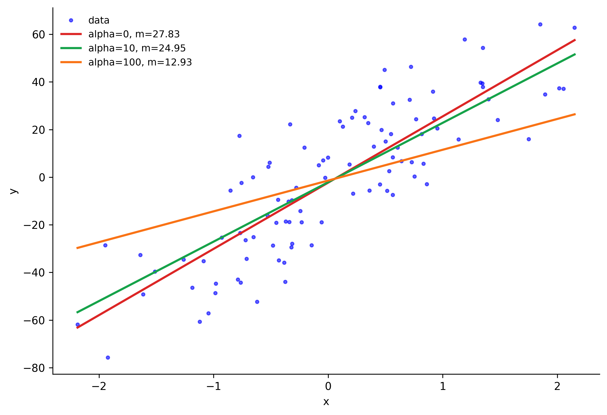
The red alpha=0 line has the steepest slope and passes closest through the bulk of the points. The green alpha=10 line is visibly shallower, and the orange alpha=100 line is shallower still, on its way toward flattening into a horizontal line predicting the mean as $\lambda \to \infty$.

3. Coding the Formula from Scratch

class MeraRidge:
 
    def __init__(self, alpha=0.1):
        self.alpha = alpha
        self.m = None
        self.b = None
 
    def fit(self, X_train, y_train):
        num = 0
        den = 0
 
        for i in range(X_train.shape[0]):
            num = num + (y_train[i] - y_train.mean()) * (X_train[i] - X_train.mean())
            den = den + (X_train[i] - X_train.mean()) * (X_train[i] - X_train.mean())
 
        self.m = num / (den + self.alpha)
        self.b = y_train.mean() - (self.m * X_train.mean())

Running MeraRidge(alpha=10).fit(X, y) prints m=24.95, b=-2.13, and MeraRidge(alpha=100).fit(X, y) prints m=12.93, b=-1.42, matching Ridge to four decimal places. The formula holds.

4. Extending to n Dimensions: The Matrix Form

The single-feature derivation doesn't scale to datasets with multiple features. For that, the loss needs to be written in matrix form, the same way Ch.6 rewrote plain multiple linear regression before deriving its closed-form solution.

Stack the $n$ training rows into a design matrix $X$ (with a leading column of ones for the intercept) and the weights, including the intercept $w_0$, into a single vector $W$:

$X = \begin{bmatrix} 1 & x_{11} & \cdots & x_{1p} \\ 1 & x_{21} & \cdots & x_{2p} \\ \vdots & \vdots & & \vdots \\ 1 & x_{n1} & \cdots & x_{np} \end{bmatrix} \qquad W = \begin{bmatrix} w_0 \\ w_1 \\ \vdots \\ w_p \end{bmatrix}$

Plain linear regression's loss, $\sum (y_i - \hat y_i)^2$, becomes $(XW - Y)^T(XW - Y)$ in matrix form. Ridge adds the penalty $\lambda W^T W$ (the dot product of $W$ with itself is exactly $\sum w_j^2$):

$L = (XW - Y)^T(XW - Y) + \lambda W^T W$

Expanding the first term using $(A-B)^T = A^T - B^T$:

$L = W^TX^TXW - W^TX^TY - Y^TXW + Y^TY + \lambda W^TW$

Since $W^TX^TY$ and $Y^TXW$ are both scalars and transposes of each other, they're equal, so they combine:

$L = W^TX^TXW - 2W^TX^TY + Y^TY + \lambda W^TW$

Now differentiate with respect to $W$. Two standard matrix-calculus identities are needed here:

• $\dfrac{\partial}{\partial W}(W^TAW) = 2AW$ when $A$ is symmetric (here $A = X^TX$, which is always symmetric).
• $\dfrac{\partial}{\partial W}(A^TW) = A$

Applying these term by term:

$\frac{\partial L}{\partial W} = 2X^TXW - 2X^TY + 2\lambda W = 0$

Dividing by 2 and isolating $W$:

$X^TXW + \lambda W = X^TY$

$(X^TX + \lambda I)W = X^TY$

$W = (X^TX + \lambda I)^{-1}X^TY$

This is Ridge's closed-form solution. It's the same normal equation from plain linear regression, $W = (X^TX)^{-1}X^TY$, with one change: $\lambda I$ added before inverting. $I$ here is the $(p+1) \times (p+1)$ identity matrix, matching the shape of $X^TX$.

5. Implementing the Matrix Solution

The formula translates directly into code with numpy, but there's one subtlety: the intercept $w_0$ should never be shrunk toward zero, since it's just centering the predictions, not controlling the model's sensitivity to any feature. If $\lambda I$ is applied naively, the identity matrix's [0][0] entry regularizes $w_0$ along with every other weight. The fix is to zero out that one entry before adding it in:

In the weight vector $W$, index 0 is the intercept $w_0$, not a slope, since $X$ was built with a leading column of ones. I[0][0] = 0 turns off regularization for exactly that position, so when $\lambda I$ is added to $X^TX$, $\lambda$ ends up multiplied only against the slope terms $w_1, \dots, w_p$, leaving the intercept free to shift wherever the data needs it to.

import numpy as np
 
class MeraRidge:
 
    def __init__(self, alpha=0.1):
        self.alpha = alpha
        self.coef_ = None
        self.intercept_ = None
 
    def fit(self, X_train, y_train):
        X_train = np.insert(X_train, 0, 1, axis=1)
        I = np.identity(X_train.shape[1])
        I[0][0] = 0
        result = np.linalg.inv(np.dot(X_train.T, X_train) + self.alpha * I).dot(X_train.T).dot(y_train)
        self.intercept_ = result[0]
        self.coef_ = result[1:]
 
    def predict(self, X_test):
        return np.dot(X_test, self.coef_) + self.intercept_

Testing this against sklearn.linear_model.Ridge on the diabetes dataset:

from sklearn.datasets import load_diabetes
from sklearn.model_selection import train_test_split
from sklearn.linear_model import Ridge
from sklearn.metrics import r2_score
 
X, y = load_diabetes(return_X_y=True)
X_train, X_test, y_train, y_test = train_test_split(X, y, test_size=0.2, random_state=4)
 
reg = Ridge(alpha=0.1, solver='cholesky')
reg.fit(X_train, y_train)
y_pred = reg.predict(X_test)
print(r2_score(y_test, y_pred))       # 0.4693
print(reg.coef_[:3], reg.intercept_)  # [  44.02 -241.69  452.99] 150.89
 
mera = MeraRidge(alpha=0.1)
mera.fit(X_train, y_train)
y_pred2 = mera.predict(X_test)
print(r2_score(y_test, y_pred2))         # 0.4693
print(mera.coef_[:3], mera.intercept_)   # [  44.02 -241.69  452.99] 150.89

Both the $R^2$ score and every coefficient match to the fourth decimal place. Ridge(solver='cholesky') computes the exact same closed-form matrix equation internally, just with a numerically more stable factorization than a direct matrix inverse.

6. Why This Isn't the Whole Story

The closed-form solution is exact, and there's something satisfying about deriving $(X^TX + \lambda I)^{-1}X^TY$ by hand and watching it reproduce Scikit-Learn's numbers to four decimal places. But it depends on computing $(X^TX + \lambda I)^{-1}$, a matrix inverse of a $(p+1) \times (p+1)$ matrix, which costs roughly $O(p^3)$.

That's a non-issue for the diabetes dataset's 10 features. It becomes a real bottleneck once $p$ climbs into the thousands, the kind of feature counts common with one-hot encoded categorical data or bag-of-words text representations. At that scale, computing a matrix inverse directly stops being practical.

The next post covers the alternative: solving the same regularized loss with gradient descent instead of a direct matrix inversion, the same iterative approach from Ch.7 adapted to include the $\lambda$ term in the gradient update.