Ch.21: Coding the Perceptron Trick (And Why It's Not Enough)

Inspired by: YouTube

Ch.20 worked out the Perceptron Trick's logic: represent a line as a weight vector, loop over random points, nudge the line toward whichever one it's currently getting wrong. This post codes that algorithm and then uses the finished implementation to expose exactly why real Logistic Regression needs to be a different, more careful algorithm.

1. Implementing the Perceptron Trick

import numpy as np
from sklearn.datasets import make_classification
 
X, y = make_classification(n_samples=100, n_features=2, n_informative=1, n_redundant=0,
                            n_classes=2, n_clusters_per_class=1, random_state=41,
                            hypercube=False, class_sep=10)
 
def step(z):
    return 1 if z > 0 else 0
 
def perceptron(X, y, epochs=1000, lr=0.1):
    X = np.insert(X, 0, 1, axis=1)
    weights = np.ones(X.shape[1])
 
    for i in range(epochs):
        j = np.random.randint(0, 100)
        y_hat = step(np.dot(X[j], weights))
        weights = weights + lr * (y[j] - y_hat) * X[j]
 
    return weights[0], weights[1:]

Every line traces straight back to Ch.20's derivation:

• np.insert(X, 0, 1, axis=1) prepends the constant x_0=1 column, so the intercept becomes just another weight instead of a special case.
• weights = np.ones(...) starts from an arbitrary line, here all 1s.
• Each loop iteration picks one random training row (j), computes that row's current prediction with step(np.dot(X[j], weights)), and applies the unified update rule $W \mathrel{+}= \eta(y-\hat y)X$ in a single line, no if branch needed since $y-\hat y$ is already 0 for correctly classified points.

Running it: perceptron(X, y) returns an intercept and a two-element coefficient array, the same (w0, w1, w2) split used throughout the Ridge and Lasso posts' closed-form derivations.

2. Converting Weights Back to a Plottable Line

weights isn't directly a slope and intercept, it's the $(w_0, w_1, w_2)$ from $w_0 + w_1 x_1 + w_2 x_2 = 0$. Solving that for $x_2$ in terms of $x_1$ recovers the familiar $y=mx+b$ form:

def line_mb(intercept, coef):
    m = -(coef[0] / coef[1])
    b = -(intercept / coef[1])
    return m, b

Plotting this line against the training data confirms it separates the two classes, matching the result from Ch.20's before-after comparison: the perceptron trick, run for enough epochs on linearly separable data, reliably lands on a working separating line.

3. The Real Test: Compare Against Scikit-Learn's LogisticRegression

Running the same dataset through sklearn.linear_model.LogisticRegression and plotting both lines together is where the perceptron trick's actual weakness shows up:

from sklearn.linear_model import LogisticRegression
 
intercept_, coef_ = perceptron(X, y)
m_p, b_p = line_mb(intercept_, coef_)
 
lor = LogisticRegression()
lor.fit(X, y)
m_l, b_l = line_mb(lor.intercept_[0], lor.coef_[0])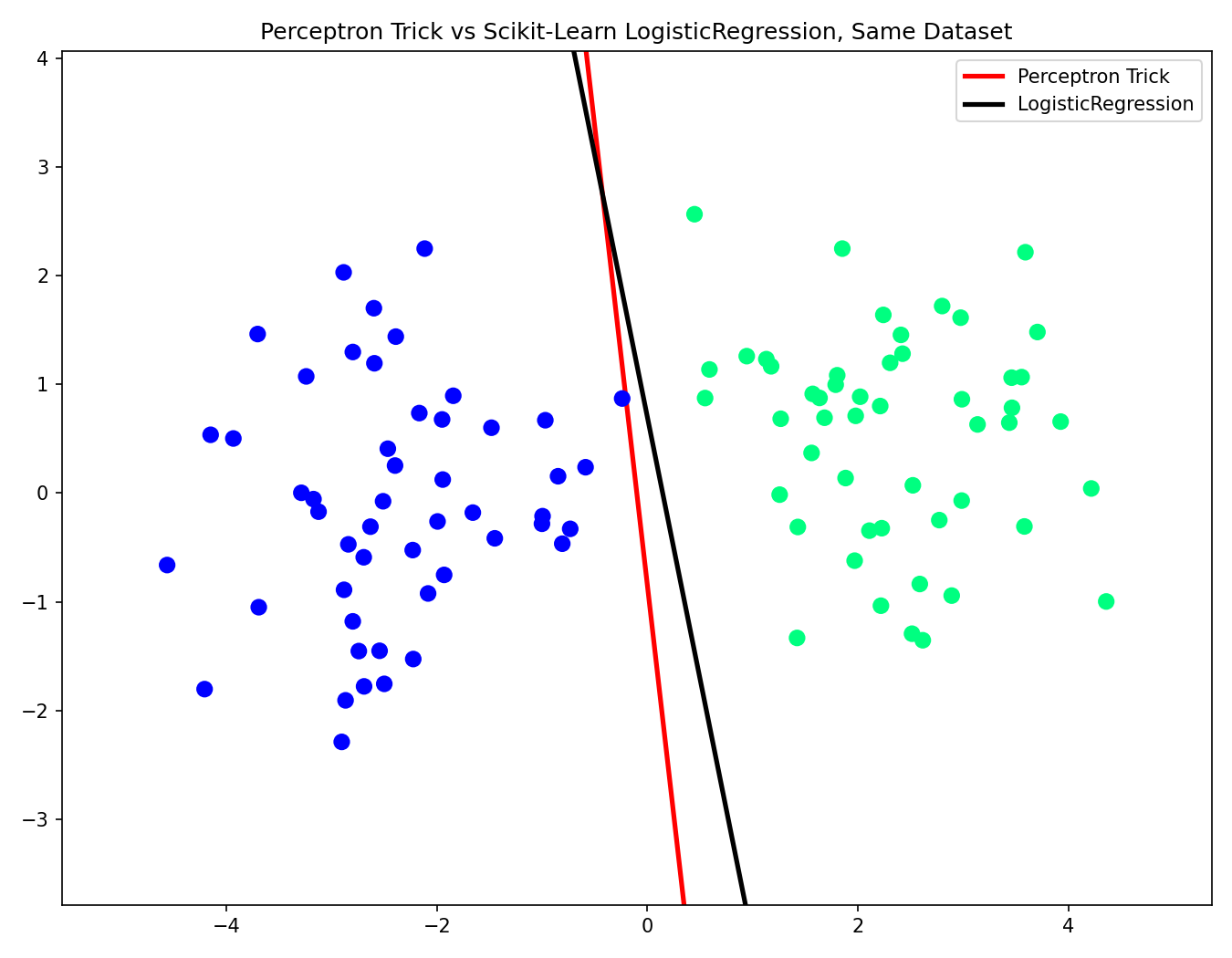

Both lines get every point right, zero training errors each. But they're clearly not the same line. The red perceptron line passes close enough to one of the blue points that it barely counts as separating it, no breathing room at all on that side. The black Logistic Regression line sits further over, leaving a visibly wider gap between itself and both clusters, a much more comfortable, symmetric-looking boundary.

4. Why the Two Lines Differ

The perceptron trick's stopping condition is simple: keep nudging until no point is misclassified, then stop. The instant every training point lands on the correct side, the loop has nothing left to fix, and whatever line happens to be in place at that exact moment becomes the final answer, even if it's only barely separating the classes with almost no margin to spare.

Logistic Regression's training process doesn't stop there. It keeps adjusting the line even after every point is already correctly classified, because it isn't minimizing "number of misclassified points", it's minimizing a smooth loss function (built from probabilities, the subject of the next post) that keeps rewarding a wider, more confident margin between the line and both classes. That difference, stop at merely correct versus keep improving toward confidently correct, is the entire gap between the red and black lines above.

5. Why This Matters: Generalization

A separating line that barely squeezes past one class, the way the perceptron trick's line does, is fragile. A new, unseen data point that lands only slightly to the left of where that blue point sits, still well inside where a human would call "obviously the blue cluster", could easily fall on the wrong side of a line with that little margin. The wider-margin black line has more slack: nearby new points are more likely to land on the correct side, because the line isn't hugging the training data as tightly.

This is the practical reason the perceptron trick, while a genuinely useful stepping stone for building intuition, isn't what real classifiers use in practice. It solves an easier problem (find any separating line) instead of the one that actually matters for generalizing to new data (find the best separating line). The next post picks up exactly here: reformulating the problem with an actual loss function so that "best" has a precise, optimizable meaning, arriving at Logistic Regression's real training procedure.