Ch.7: Gradient Descent - Intuition, Math, and Implementation

Inspired by: YouTube

Ch.1 and Ch.2 derived the closed-form Ordinary Least Squares (OLS) solution for simple linear regression. Ch.3 and Ch.4 covered evaluation metrics and core diagnostic assumptions. Ch.5 and Ch.6 extended linear regression to $k$ features using matrix algebra, solving for parameters directly with the closed-form normal equation $\hat{\beta} = (X^T X)^{-1} X^T y$.

In this post, we introduce Gradient Descent, the foundational optimization algorithm that powers modern machine learning and deep learning. We examine why gradient descent is essential when closed-form solutions become computationally intractable, derive its partial derivatives step by step, animate its convergence live, build a custom estimator from scratch in Python, and analyze the impact of learning rate and epochs.

Why Gradient Descent Matters: Beyond Closed-Form Solutions

In the previous post on multiple linear regression math, we solved for parameter vector $\beta$ using the normal equation:

$\hat{\beta} = (X^T X)^{-1} X^T y$

While mathematically elegant, the normal equation suffers from a severe computational limitation: matrix inversion. For a dataset with $n$ rows and $k$ features, the matrix $X^T X$ has dimensions $(k+1) \times (k+1)$. Inverting a matrix of shape $(k, k)$ requires roughly $\mathcal{O}(k^3)$ operations (or $\mathcal{O}(k^{2.81})$ using Strassen's algorithm).

When feature count $k$ is small (e.g., $k = 10$ or $k = 100$), matrix inversion completes in milliseconds. However, when working with high-dimensional datasets such as text embeddings, genomic data, or image pixels where $k$ reaches $100{,}000$ or $1{,}000{,}000$, computing $(X^T X)^{-1}$ requires extreme computational time and exceeds available RAM.

Furthermore, closed-form solutions exist only for a small family of algorithms like linear regression. Non-linear models, logistic regression, Support Vector Machines, and Deep Neural Networks do not have closed-form solutions.

Gradient descent solves both problems. Instead of calculating optimal parameters in a single massive matrix calculation, gradient descent starts with arbitrary initial guesses and iteratively steps down the loss function surface until it converges to the optimal solution.

1D Intuition: Fixing Slope $m$ and Optimizing Intercept $b$

To build intuition, consider simple linear regression $y = m x + b$. Suppose slope $m$ is fixed to a known constant (e.g., $m = 27.83$). The model must optimize a single parameter: intercept $b$.

The objective is to minimize the Sum of Squared Errors (SSE) loss function $L(b)$:

$L(b) = \sum_{i=1}^n \left(y_i - (m x_i + b)\right)^2$

Because $L(b)$ is a quadratic function of $b$, plotting $L(b)$ against $b$ creates a 1D convex parabola with a single global minimum $b^*$.

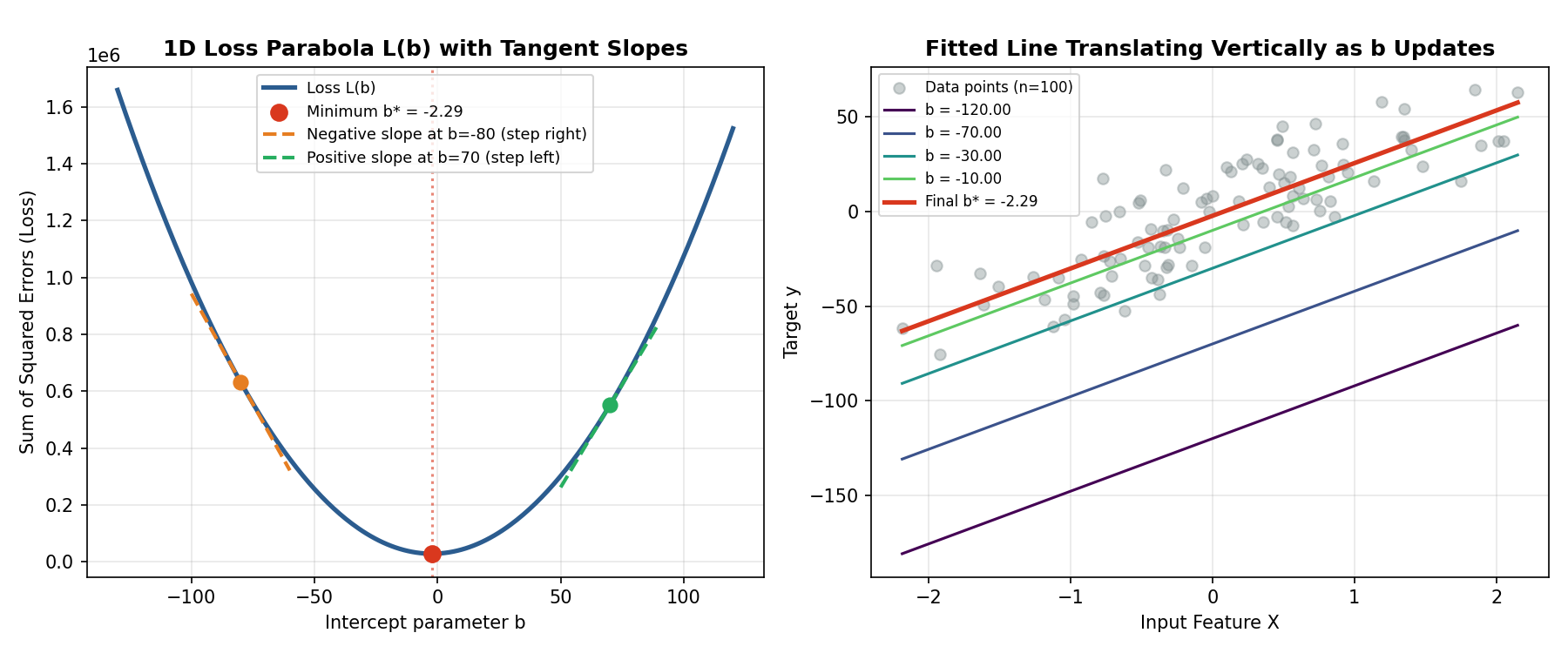
Imagine standing on this loss parabola blindfolded. You cannot view the whole curve, but you can feel the local incline (the derivative or slope of the tangent line):

1. If you start at $b_0 = -80$ (left side of minimum): The tangent slope $\frac{\mathrm{d}L}{\mathrm{d}b}$ is negative. To move closer to the minimum $b^*$, you must increase $b$ (step to the right).
2. If you start at $b_0 = 70$ (right side of minimum): The tangent slope $\frac{\mathrm{d}L}{\mathrm{d}b}$ is positive. To move closer to the minimum $b^*$, you must decrease $b$ (step to the left).

This yields the fundamental update rule:

$b_{\text{new}} = b_{\text{old}} - \eta \cdot \frac{\mathrm{d}L}{\mathrm{d}b}$

where $\eta$ (eta) is the learning rate, a small positive scalar (e.g., $\eta = 0.001$). The minus sign automatically handles direction:

• When slope is negative ($\frac{\mathrm{d}L}{\mathrm{d}b} < 0$), subtracting a negative quantity adds to $b_{\text{old}}$, moving $b$ rightward.
• When slope is positive ($\frac{\mathrm{d}L}{\mathrm{d}b} > 0$), subtracting a positive quantity reduces $b_{\text{old}}$, moving $b$ leftward.

Batch Gradient Descent Derivation for $m$ and $b$

Now consider the full simple linear regression problem where both slope $m$ and intercept $b$ are unknown.

The target model is $\hat{y}_i = m x_i + b$. The total loss across all $n$ data points is:

$L(m, b) = \sum_{i=1}^n \left(y_i - (m x_i + b)\right)^2$

Because $L(m, b)$ depends on two parameters, the loss function forms a 3D bowl-shaped surface (a paraboloid). To find the direction of steepest descent, we compute the gradient vector $\nabla L(m, b)$, which contains partial derivatives with respect to each parameter.

That surface is the real cost function $L(m, b)$ for this exact dataset, drag to rotate, scroll to zoom. The orange trail is the actual batch gradient descent path from the 60-epoch run below, stepping from the starting guess down the bowl to the global minimum.

Deriving the Partial Derivative w.r.t Intercept $b$

Using the chain rule:

$\frac{\partial L}{\partial b} = \frac{\partial}{\partial b} \sum_{i=1}^n \left(y_i - m x_i - b\right)^2$

Bring the derivative inside the summation and apply the power rule:

$\frac{\partial L}{\partial b} = \sum_{i=1}^n 2 \left(y_i - m x_i - b\right) \cdot \frac{\partial}{\partial b}\left(y_i - m x_i - b\right)$

Since $\frac{\partial}{\partial b}(y_i - m x_i - b) = -1$:

$\frac{\partial L}{\partial b} = -2 \sum_{i=1}^n \left(y_i - (m x_i + b)\right) = -2 \sum_{i=1}^n (y_i - \hat{y}_i)$

Deriving the Partial Derivative w.r.t Slope $m$

Similarly, differentiate $L(m, b)$ with respect to $m$:

$\frac{\partial L}{\partial m} = \frac{\partial}{\partial m} \sum_{i=1}^n \left(y_i - m x_i - b\right)^2$

Apply the chain rule:

$\frac{\partial L}{\partial m} = \sum_{i=1}^n 2 \left(y_i - m x_i - b\right) \cdot \frac{\partial}{\partial m}\left(y_i - m x_i - b\right)$

Since $\frac{\partial}{\partial m}(y_i - m x_i - b) = -x_i$:

$\frac{\partial L}{\partial m} = -2 \sum_{i=1}^n \left(y_i - (m x_i + b)\right) x_i = -2 \sum_{i=1}^n (y_i - \hat{y}_i) x_i$

Simultaneous Parameter Update Rules

At each epoch $k$, both parameters are updated simultaneously using their respective partial derivatives and learning rate $\eta$:

$b^{(k+1)} = b^{(k)} - \eta \cdot \left( -2 \sum_{i=1}^n (y_i - \hat{y}_i) \right)$

$m^{(k+1)} = m^{(k)} - \eta \cdot \left( -2 \sum_{i=1}^n (y_i - \hat{y}_i) x_i \right)$

Notice how step size is governed by gradient magnitude. Far from the minimum, residuals $(y_i - \hat{y}_i)$ and gradients are large, producing larger initial steps. As parameters approach optimal values $(m^*, b^*)$, gradients diminish toward zero, naturally slowing step sizes so the algorithm settles cleanly into the minimum.

Live Convergence Animation

The interactive component below demonstrates 60 epochs of batch gradient descent starting from initial parameters $m_0 = 100, b_0 = -120$ with learning rate $\eta = 0.001$. Watch the fitted line rotate and translate in real time as the cost curve drops smoothly toward zero.

Building GDRegressor from Scratch in Python

We validate our derivation by constructing a custom estimator class named GDRegressor, following the implementation structure in the source notebook gradient-descent-code-from-scratch.ipynb.

We generate a synthetic regression dataset using sklearn.datasets.make_regression with 100 samples, 1 feature, noise level 20, and random_state=13.

import numpy as np
import matplotlib.pyplot as plt
from sklearn.datasets import make_regression
from sklearn.linear_model import LinearRegression
 
# Generate synthetic dataset matching source notebook
X, y = make_regression(
    n_samples=100, 
    n_features=1, 
    n_informative=1, 
    n_targets=1, 
    noise=20, 
    random_state=13
)
 
# Benchmark using scikit-learn's OLS LinearRegression
ols = LinearRegression()
ols.fit(X, y)
 
print(f"OLS Slope (m): {ols.coef_[0]:.2f}")
print(f"OLS Intercept (b): {ols.intercept_:.2f}")
# Output:
# OLS Slope (m): 27.83
# OLS Intercept (b): -2.29

Now we build the custom GDRegressor class implementing batch gradient descent:

class GDRegressor:
    def __init__(self, learning_rate=0.001, epochs=100):
        self.lr = learning_rate
        self.epochs = epochs
        # Initial guesses far from true values (m=27.83, b=-2.29)
        self.m = 100.0
        self.b = -120.0
 
    def fit(self, X, y):
        X_ravel = X.ravel()
        n_samples = len(y)
 
        for epoch in range(self.epochs):
            # Compute current predictions
            y_pred = self.m * X_ravel + self.b
            
            # Compute partial derivatives (Sum of Squared Errors)
            loss_slope_b = -2 * np.sum(y - y_pred)
            loss_slope_m = -2 * np.sum((y - y_pred) * X_ravel)
 
            # Update parameters simultaneously
            self.b = self.b - self.lr * loss_slope_b
            self.m = self.m - self.lr * loss_slope_m
 
    def predict(self, X):
        return self.m * X.ravel() + self.b

We instantiate GDRegressor, fit it on the exact same dataset, and print the converged parameters:

# Instantiate and fit custom estimator
gd = GDRegressor(learning_rate=0.001, epochs=100)
gd.fit(X, y)
 
print(f"GD Slope (m): {gd.m:.2f}")
print(f"GD Intercept (b): {gd.b:.2f}")
# Output:
# GD Slope (m): 27.83
# GD Intercept (b): -2.29

Our from-scratch gradient descent implementation converges to $m = 27.83$ and $b = -2.29$, matching scikit-learn's OLS values to two decimal places.

Conceptual Analysis: Learning Rate and Epochs

The performance and stability of gradient descent depend directly on two key hyperparameters: learning rate $\eta$ and number of epochs.

Impact of Learning Rate ($\eta$)

The tool below fixes slope $m$ at its optimal value (the same 1D slice from earlier) and lets you drive gradient descent on $b$ by hand: drag the learning rate slider, hit Step to take one update, and watch where the orange marker lands on the loss curve.

Because this 1D slice is an exact parabola, the update has a closed form: $b^{(k+1)} - b^* = (1 - 2\eta n)(b^{(k)} - b^*)$, where $n = 100$ is the sample count. That geometric recurrence converges only when $|1 - 2\eta n| < 1$, i.e. $\eta < \frac{1}{n} = 0.01$ for this dataset:

1. Learning Rate Too Small ($\eta \approx 0.0005$): $(1 - 2\eta n)$ sits close to 1, so each step shrinks the distance to $b^*$ by only a sliver. The algorithm needs hundreds of steps to make visible progress, crawling slowly down the loss curve. Safe, but wasteful.
2. Optimal Learning Rate ($\eta \approx 0.004$): Steps are well-sized. Loss drops smoothly every step and settles at the minimum within a handful of clicks.
3. Learning Rate Too Large ($\eta \geq 0.01$): $|1 - 2\eta n|$ crosses 1, so each step overshoots $b^*$ by a larger margin than the last. Instead of descending, $b$ bounces between opposite walls of the parabola with growing amplitude, and loss explodes toward infinity, exactly the "will never reach the minimum" case the tool warns about.

Impact of Epochs

An epoch represents one full iteration over the training dataset.

• If epochs are too low (e.g., 5 epochs), training stops prematurely before parameters reach the minimum (underfitting).
• As epochs increase, parameter changes $\Delta m = |m^{(k+1)} - m^{(k)}|$ and $\Delta b = |b^{(k+1)} - b^{(k)}|$ shrink toward zero.
• Practical stopping criteria include setting a fixed max epoch budget or monitoring convergence: stopping early when $|L^{(k+1)} - L^{(k)}| < \epsilon$ (where $\epsilon = 10^{-5}$).

Why Feature Scaling Speeds Up Convergence

Picture the loss surface as a valley, and gradient descent as walking downhill toward its lowest point. If every feature is on a similar scale, that valley is a nice round bowl, and a single step size works equally well no matter which direction you're walking. But if one feature ranges from 0 to 1 and another ranges from 0 to 100,000, the bowl gets stretched into a long, narrow canyon: steep, cliff-like walls along the large-scale feature's axis, and an almost flat, gentle slope along the small-scale one.

Gradient descent only has one step size (the learning rate $\eta$), and it has to use that same step size in every direction at once. To avoid overshooting and bouncing off the steep canyon walls, $\eta$ has to be kept small, but that same small $\eta$ makes it crawl along the gentle slope. So instead of walking straight down to the bottom, it zig-zags back and forth across the narrow direction while barely creeping forward along the wide one, taking far more steps than it should to actually get anywhere.

Formally: for MSE-style loss, the curvature of $L$ along a weight's axis scales with that feature's variance, since the Hessian is $2 X^T X$, and the diagonal entry for feature $j$ is approximately $2n \cdot \sigma_j^2$. If one feature's standard deviation is $5\times$ another's, its axis carries roughly $25\times$ more curvature, which is exactly the steep-canyon-vs-gentle-slope mismatch described above, just measured precisely instead of by eye.

Both panels above run real gradient descent for 40 steps from the same starting point, on quadratic bowls $L(w_1, w_2) = a w_1^2 + b w_2^2$ that model this curvature relationship directly. With $a{:}b = 25{:}1$ (mimicking a $5{:}1$ feature standard-deviation ratio), the largest stable learning rate is dictated by $a$, and $w_2$ is still at $0.274$ after 40 steps while $w_1$ has already oscillated its way to convergence. Standardizing so both features have unit variance ($a = b = 1$) makes the bowl circular: the same 40-step budget with a much larger learning rate lands within $10^{-16}$ of the minimum, no zig-zag required.

This is why StandardScaler (subtracting the mean, dividing by the standard deviation) is standard practice before gradient-based training, closed-form OLS doesn't care about feature scale since it solves for the minimum directly, but gradient descent's convergence speed depends heavily on it.

Non-Convex Loss Surfaces and the Saddle Point Problem

Every loss surface in this post so far has been a convex bowl (a paraboloid) with exactly one minimum, which is guaranteed for linear regression's squared-error loss: no matter where gradient descent starts, it eventually reaches the same global optimum. Logistic regression, neural networks, and most other models people apply gradient descent to do not get this guarantee. Their loss surfaces can be non-convex: full of dips, ridges, and flat regions where the same algorithm behaves very differently depending on where it starts.

A minimal function that captures this is $f(x, y) = x^4 - 2x^2 + y^2$. Setting both partial derivatives to zero, $\frac{\partial f}{\partial x} = 4x^3 - 4x = 4x(x^2 - 1) = 0$ and $\frac{\partial f}{\partial y} = 2y = 0$, gives three critical points: $(-1, 0)$, $(0, 0)$, and $(1, 0)$. Checking the second derivative along $x$, $\frac{\partial^2 f}{\partial x^2} = 12x^2 - 4$, shows $(\pm 1, 0)$ are curved upward ($+8$, a local minimum along $x$) while $(0, 0)$ is curved downward ($-4$, a local maximum along $x$). Combined with $y^2$ always curving upward along $y$, the origin is concave in one direction and convex in the other: a saddle point, not a minimum, even though its gradient is exactly zero there.

The plot runs real batch gradient descent (learning rate $0.05$, analytic gradients, no approximation) from three starting points on this exact surface. Paths starting clearly to one side of the saddle converge quickly, reaching within $10^{-4}$ of a global minimum in around 15 steps. The path starting almost directly above the saddle at $(0.01, 1.0)$ behaves very differently: $x$ crawls from $0.01$ to only $0.06$ over the first 10 steps, because the gradient $4x(x^2-1)$ is nearly zero when $x$ is near zero. It takes roughly 30 steps of this near-flat plateau before $x$ escapes and accelerates into the same basin the direct paths reached in half the time.

This is the practical saddle point problem: near a saddle, the gradient magnitude shrinks toward zero just like it does near a true minimum, so a plain fixed-step gradient descent update slows to a crawl without actually being close to done. In low dimensions like this 2D example, the descent does eventually escape (a random or off-axis start almost never lands exactly on the unstable direction). In the very high-dimensional loss landscapes typical of neural networks, saddle points vastly outnumber true local minima, which is part of why optimizers used in practice (momentum, Adam, and similar) add mechanisms specifically to accelerate through these flat, low-gradient regions rather than relying on plain gradient descent alone.

Summary & Key Takeaways

1. Why Gradient Descent: Matrix inversion in the OLS normal equation scales as $\mathcal{O}(k^3)$, making it computationally intractable for large feature counts. Gradient descent scales as $\mathcal{O}(k \cdot n)$ per epoch and generalizes to non-linear models and deep learning.
2. Direction via Derivative: The negative gradient direction $-\nabla L$ always points toward steepest loss reduction. The minus sign in $p_{\text{new}} = p_{\text{old}} - \eta \cdot \frac{\partial L}{\partial p}$ ensures updates move opposite to the gradient.
3. Partial Derivatives: For SSE loss $L(m, b) = \sum (y_i - (m x_i + b))^2$, partial derivatives are $\frac{\partial L}{\partial b} = -2 \sum (y_i - \hat{y}_i)$ and $\frac{\partial L}{\partial m} = -2 \sum (y_i - \hat{y}_i) x_i$.
4. Hyperparameter Tuning: Learning rate $\eta$ controls step size. Too small leads to slow convergence; too large causes oscillation and divergence.
5. Exact OLS Match: Our custom GDRegressor built from scratch converges to $m = 27.83, b = -2.29$ on synthetic data, matching scikit-learn's LinearRegression benchmark.
6. Feature Scaling: Loss curvature scales with feature variance, so unscaled features stretch the loss surface into thin ellipses. A single global learning rate then zig-zags on the steep axis while crawling on the shallow one; standardizing features to unit variance makes the surface circular and convergence direct.
7. Non-Convexity and Saddle Points: Linear regression's loss is convex with one guaranteed global minimum, but models like neural networks have non-convex loss surfaces with local minima and saddle points, flat regions with zero gradient that aren't minima, where plain gradient descent slows to a crawl before escaping.

In the next post, we explore variants of gradient descent (Batch, Stochastic, and Mini-Batch Gradient Descent) to optimize performance on massive datasets.