
Ch.37: The Curse of Dimensionality, Feature Selection, and Feature Extraction
Inspired by: YouTube
In the previous post, we covered Feature Construction and Feature Splitting, the two manual, intuition-driven branches of feature engineering. With those complete, we have now finished the first two pillars of the feature engineering tree: Feature Transformation (scaling, encoding, missing values, outliers) and Feature Construction (creating new columns from domain knowledge).
This post introduces the remaining two pillars: Feature Selection and Feature Extraction. Both exist to solve a single underlying problem that becomes unavoidable as your feature count grows: the Curse of Dimensionality.
The Curse of Dimensionality
More Features ≠ Better Models
A common misconception, especially early on, is that feeding a model more features will always improve its predictions. Intuitively this sounds right: more information should help, not hurt. But in practice, model performance follows a curve that rises, plateaus, and then falls as the number of features increases.
There exists an optimal number of features for any given model and dataset. Up to that point, each new feature contributes useful signal and accuracy improves. Beyond it, additional features add more noise than signal, computational cost climbs, and the model's ability to generalize degrades. This phenomenon, where high-dimensional feature spaces actively hurt model performance, is what is meant by the Curse of Dimensionality.
To make this concrete, the chart below runs a small real experiment: a synthetic 60-feature dataset (12 informative, 8 redundant, the rest pure noise) with a KNN classifier (k=5), retrained repeatedly while feeding it more and more of those features in order:
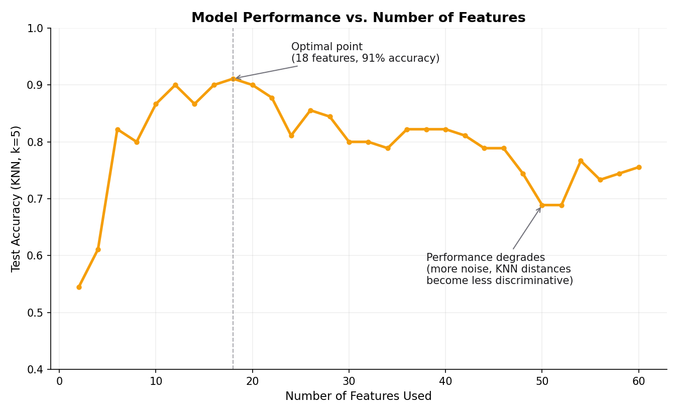
Accuracy climbs sharply as the first informative features are added, peaks once the 12 informative and 8 redundant columns are all in play, then drops as the remaining pure-noise columns get mixed in. KNN's decisions get worse not because the informative signal disappeared, but because computing distance across dozens of irrelevant dimensions drowns it out.
Three concrete problems emerge as dimensionality grows:
- Performance plateau and decline. Beyond the optimal feature count, the model starts memorizing noise rather than learning signal. Generalization error increases.
- Computational cost explodes. Training time, memory usage, and prediction latency all scale with the number of features. A model with 784 features takes dramatically more resources than one with 50, even if those extra 734 features contribute nothing.
- Distance metrics become meaningless. Many algorithms (KNN, SVM with RBF kernels, clustering methods) rely on computing distances between data points. In high-dimensional space, a counterintuitive phenomenon occurs: all points become approximately equidistant from each other. When every point is roughly the same distance from every other point, the concept of "nearest neighbor" loses its discriminative power, and distance-based algorithms fail.
Why High-Dimensional Distance Breaks Down
To build intuition for this, think of a concrete analogy: you have lost your wallet, and you're told which space it's somewhere in.
- 1D: somewhere on the road from the college gate to the college building. A road is a line. You just walk its length once, checking as you go. Trivial.
- 2D: somewhere in a park. Now you're searching an area, not a line. You have to sweep back and forth across two dimensions of open ground, a search that takes meaningfully longer than walking a single road of the same length.
- 3D: somewhere inside the college building. Now you're searching a volume: every floor, every room, every corridor. The building occupies roughly the same footprint as the park, but because you've added a third dimension (height, floors), the number of distinct places the wallet could be has exploded far beyond the park's.
The wallet hasn't moved, and the search area's rough footprint hasn't changed much either. What changed is the dimensionality of the space it's hidden in, and that alone made the search dramatically harder. Each dimension you add multiplies the number of places to check, not adds to it.
The same thing happens with data. In one or two dimensions, data points cluster naturally into groups that are easy to separate. As you add more and more dimensions, the data points spread out into an increasingly vast space, and the available data becomes sparse relative to it.
Why "Nearest" Neighbor Loses Meaning
Sparsity explains why data gets spread thin, but it doesn't yet explain the sharper claim from earlier: that the nearest point and the farthest point start to look the same. That takes one more step of intuition.
Picture comparing people using a single feature, height. Whoever's height is closest to yours is unambiguously your nearest neighbor. Simple, one number decides it.
Now add a second, independent feature: weight. Distance is now . A pair that differs a lot in height but happens to match closely in weight can now land at roughly the same total distance as a pair that differs only a little in height but a lot in weight. Two genuinely different-looking pairs can now produce the same number.
Keep adding independent features, age, income, shoe size, blood pressure, GPA, hundreds of them. Each one contributes its own small, mostly unrelated difference to the running total. This is exactly the situation an average lives in: flip one coin and you might get heads or tails, pure luck either way; flip a thousand coins and the total lands very close to 500 heads almost every time, because the individual swings cancel each other out. Distance across many independent features behaves the same way: no single feature can any longer swing the total decisively, because it's just one of hundreds of contributors being summed, and that sum settles toward a similar, typical value for every pair of points, whether they're genuinely alike or not.
That's the actual mechanism: nearest and farthest neighbor both drift toward that same typical distance, so the gap between them, the exact gap that KNN depends on to mean anything, shrinks toward nothing.
This isn't hand-waving, it's directly measurable. The chart below fixes a query point and scatters 2,000 random points in a unit hypercube, then tracks as dimensionality climbs from 1 to 5,000:
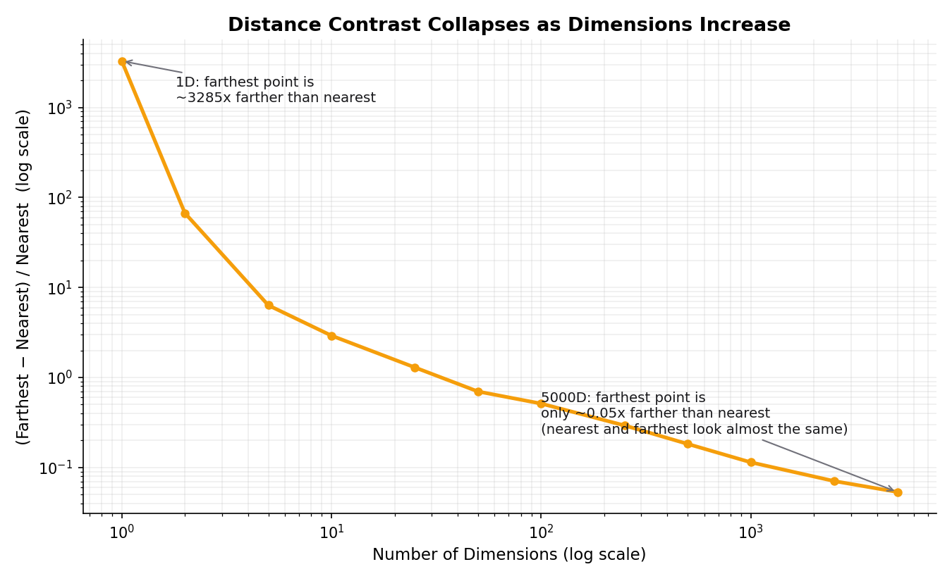
At 1 dimension, the farthest point is over 3,000x farther away than the nearest, a huge, unambiguous gap. By 5,000 dimensions, that gap has collapsed to roughly 0.05x, the farthest point is barely 5% farther than the nearest. Every point has become almost equidistant from the query, exactly as the coin-flip intuition predicts. This is why KNN, RBF-kernel SVMs, and distance-based clustering all degrade as dimensionality grows: their core assumption, that distance is a meaningful measure of similarity, quietly stops being true.
The MNIST Example: 784 Features for Handwritten Digits
To see why this matters concretely, consider the classic MNIST handwritten digit dataset. Each image is 28 × 28 pixels. When flattened into a tabular row for a machine learning model, that single image becomes a vector of 784 features (one per pixel).
But are all 784 features equally useful? Not even close. As we demonstrated back in Ch.14: Introduction to Feature Engineering, the border pixels of these images are almost always white (value 0) across every digit sample. They have near-zero variance, which means they carry no discriminative information whatsoever. The actual digit strokes are concentrated in the central region of the image.
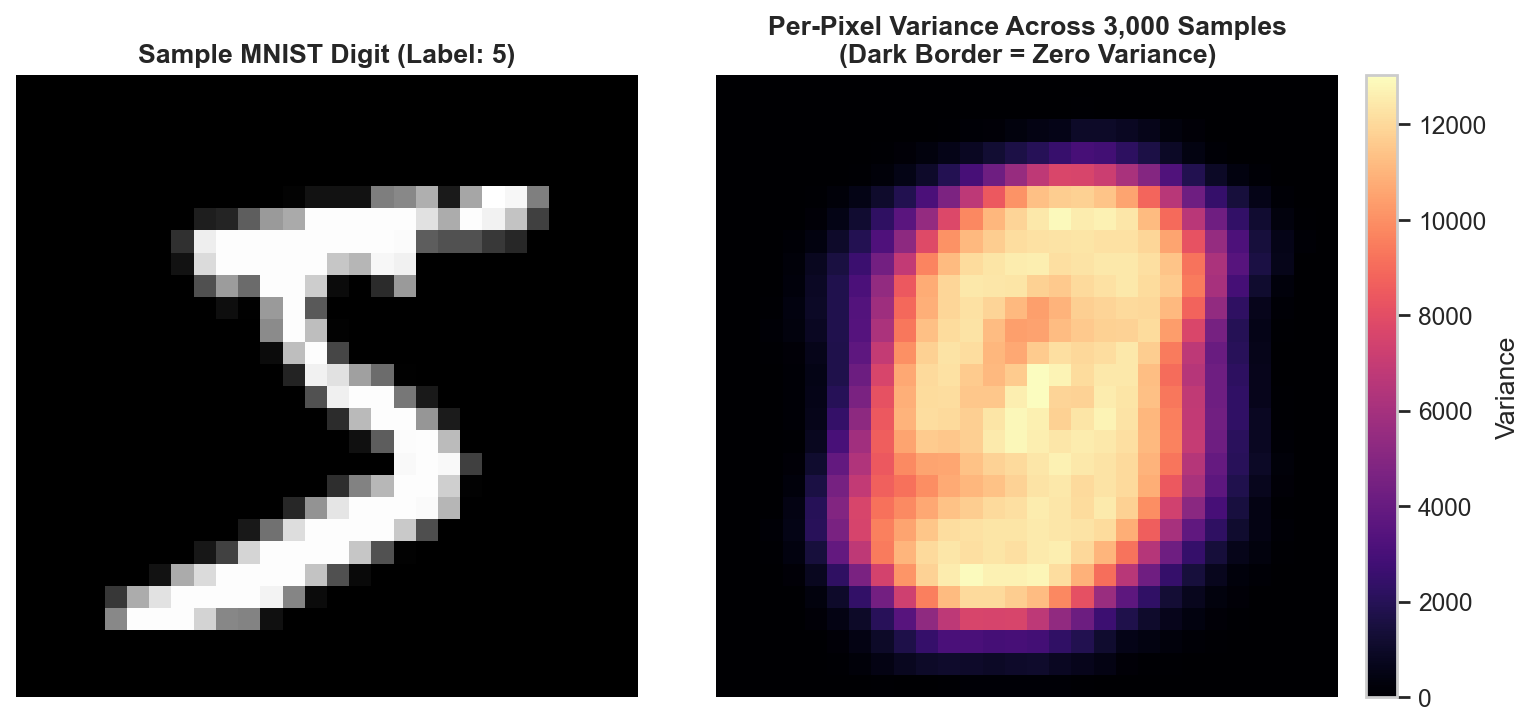
The heatmap above (from Ch.14) makes this obvious: border pixels are dark (zero variance), center pixels are bright (high variance). If your model ingests all 784 features, the several hundred zero-variance border pixels contribute nothing to accuracy while increasing training time, memory consumption, and the risk of overfitting. The model has to process and carry weights for columns that are pure dead weight.
This is the Curse of Dimensionality in action on a real dataset. The question then becomes: how do we get rid of the useless dimensions while keeping the useful ones?
Two Paths to Reducing Dimensionality
There are two fundamentally different strategies for reducing the number of features. Both reduce dimensionality, but they work in very different ways:
Feature Selection: Choosing What to Keep
Feature Selection takes the original set of features and selects a subset of them, discarding the rest. The features that survive are untouched: they are the same columns with the same values, just fewer of them.
Going back to the MNIST example: if you run variance analysis across all 784 pixel columns and find that 300 of them have near-zero variance (the border pixels), you can simply drop those 300 columns and train your model on the remaining 484. Each retained column is still an original pixel value, perfectly interpretable and unchanged.
Common Feature Selection techniques include:
- Variance Threshold: drop columns whose variance falls below a cutoff.
- Univariate Statistical Tests: rank features by their individual correlation or mutual information with the target variable and keep the top-k.
- Forward/Backward Selection: iteratively add or remove features based on model performance.
- Feature Importance from Models: train a model (e.g., Random Forest) and rank features by their learned importance scores.
The key advantage of Feature Selection is interpretability: the surviving features are the same columns you started with, so you can always explain what the model is looking at. The disadvantage is that you might lose information carried by the dropped features.
Feature Extraction: Creating Something New
Feature Extraction takes a different approach. Instead of choosing among existing features, it creates entirely new features that are mathematical combinations of the originals. These new features are designed to compress the maximum amount of information from the original high-dimensional space into a much smaller number of dimensions.
The most important technique in this category is Principal Component Analysis (PCA). PCA finds the directions (axes) of maximum variance in the data and projects all data points onto those axes. The result is a set of new "principal components," each of which is a weighted combination of every original feature, ranked by how much variance they capture.
For MNIST, instead of selecting 484 of the 784 original pixels, PCA might produce 50 principal components that together capture 95% of the total variance in the dataset. Each component blends information from all 784 pixels into a single synthetic variable.
As shown in Ch.14, even a simple dataset like Iris (4 original features) becomes visually separable when projected down to 2 principal components via PCA:
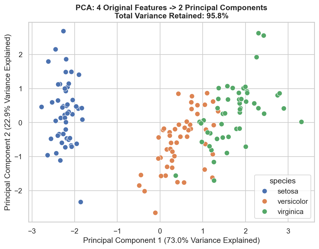
The tradeoff is the mirror image of Feature Selection: you gain a compact, information-dense representation, but you lose direct interpretability. A "principal component" is a weighted sum of all original features, so you can no longer point to a single column and say "this is pixel 342."
Feature Selection vs. Feature Extraction: When to Use Which
| Criterion | Feature Selection | Feature Extraction |
|---|---|---|
| What it produces | A subset of the original columns. | New synthetic columns (combinations of originals). |
| Interpretability | High: retained features are unchanged. | Low: components are abstract mixtures. |
| Information loss | Dropped features are completely gone. | Minimal if enough components are kept. |
| Best for | Datasets with clearly redundant or zero-variance features. | High-dimensional data (images, text, genomics) where all features carry partial signal. |
| Key techniques | Variance threshold, univariate tests, forward/backward selection, model-based importance. | PCA, LDA, t-SNE, UMAP, autoencoders. |
In practice, you might use both. For example, on MNIST you could first apply Feature Selection to drop the obvious zero-variance border pixels, then apply PCA to the remaining pixels to compress them further. The two approaches are complementary, not mutually exclusive.
Placing This in the Series
This post, and the two that precede it on Feature Construction and Feature Splitting, complete the conceptual map of all four feature engineering pillars that we first outlined in Ch.14: Introduction to Feature Engineering:
| Pillar | Status in the Series |
|---|---|
| Feature Transformation | Covered across Ch.15 through Ch.35 (scaling, encoding, missing values, outlier detection and treatment, power transforms). |
| Feature Construction | Covered in Ch.36. |
| Feature Extraction | Conceptually introduced in this post. Deep-dive with PCA coming next. |
| Feature Selection | Conceptually introduced in this post. Detailed techniques covered after ML algorithms. |
Feature Selection techniques are most naturally taught after you understand how machine learning models work, because several selection methods (forward selection, backward elimination, model-based importance) require training and evaluating a model. For that reason, the series will cover Feature Extraction (specifically PCA) next, then move into ML algorithms, and return to Feature Selection once you have the algorithmic toolkit to make sense of it.
What's Next?
In the next post, we will dive into Principal Component Analysis (PCA), the most widely used Feature Extraction technique. We will cover the mathematical intuition behind PCA (eigenvectors, eigenvalues, variance maximization), walk through a worked example, and see how PCA compresses high-dimensional data into a compact representation without discarding too much information.