
Ch.22: Power Transformer: Letting Math Pick the Best Transform for You
Inspired by: YouTube
The last post covered Mathematical Transformations: reshaping a skewed column with a fixed formula like Log or Square Root, using FunctionTransformer. Those formulas work, but you have to guess which one fits your data and try each by hand. This post covers a class that skips the guessing: PowerTransformer. Instead of applying one fixed formula, it searches for the exact exponent that makes your column look as close to a bell curve as possible, then applies it. It comes with two techniques baked in: Box-Cox and Yeo-Johnson.
A Quick Recap: Why Reshape Data At All?
Some models, like Linear Regression and Logistic Regression, work best when the numbers going into them are roughly normally distributed, meaning most values cluster near the middle and taper off evenly on both sides, like a bell curve. Real columns are rarely built that way. A column of house prices, salaries, or ingredient quantities usually has a long tail of large values dragging it off to one side. That's called being skewed.
Tree-based models like Decision Tree and Random Forest don't care about any of this, so everything in this post only matters if you're using a statistical model like Linear or Logistic Regression.
What Makes Power Transformer Different
FunctionTransformer with np.log1p applies exactly one formula: log, to every value, no matter what. That's fine, but log isn't always the best fit. Maybe your column would look more normal if you raised it to the power of 0.3, or 1.5, or some other number entirely. Trying every possible exponent by hand isn't practical.
PowerTransformer automates that search. Think of it like this: for a given column, it tries out a range of possible exponents, or "powers", checks how normal-looking the result is at each one, and keeps whichever exponent gave the best result. That best exponent is usually called lambda. Once it finds lambda, it raises every value in that column to that power. Every column gets its own lambda, tuned specifically for that column's shape.
In fact, Log Transform and Square Root Transform from the last post aren't really separate ideas: they're just two specific lambda values inside this same general family. Log is roughly what you get at lambda equal to 0, and Square Root is roughly what you get at lambda equal to 0.5. PowerTransformer doesn't force you to pick one of these ahead of time. It tries out the range and lets the data decide.
Box-Cox: The Original Version
Box-Cox is the first of the two techniques PowerTransformer supports, named after the two statisticians who came up with it. The idea: search across a range of lambda values, roughly from -5 to 5, and for each one, check how close the transformed column gets to a normal distribution. Whichever lambda produces the best-looking bell curve is the one Box-Cox keeps.
There's one important restriction to remember: Box-Cox only works on strictly positive numbers. Every value in the column has to be greater than zero. Feed it a column that contains a zero, or a negative number, and it breaks. That rules out a lot of real-world columns, since it's common for a numerical column to legitimately contain zeros.
The Box-Cox Formula
For every individual value x in a column, and a given lambda λ, the transformed value x' is computed as:
x' = (x^λ - 1) / λ      if λ ≠ 0
x' = ln(x)              if λ = 0
Where:
x: The original value, which must be strictly greater than0.λ: The exponentPowerTransformersearches for, tried across a range (roughly-5to5) to find whichever value makes the column look most normal.ln(x): The natural logarithm, used as a special case exactly whenλlands on0, since(x^0 - 1) / 0is undefined.
This is why Log Transform from the last post isn't really a separate technique: it's just what Box-Cox becomes at the specific case of λ = 0.
How does it actually find the best lambda? The short answer is a method called Maximum Likelihood Estimation, a statistical technique that shows up again and again once you get into models like Logistic Regression. There's also a separate branch of statistics, Bayesian inference, that can solve the same kind of problem differently. Both are deep topics on their own. For using
PowerTransformer, you don't need to know the internal math, just that scikit-learn's implementation is doing this search for you automatically.
Yeo-Johnson: Box-Cox Without the Restrictions
Yeo-Johnson is a newer technique, developed by two other statisticians, built specifically to remove Box-Cox's two restrictions. It can handle zero values and negative values, in addition to positive ones. Everything else about it works the same way as Box-Cox: it searches for the best lambda for each column and applies that power.
Because it works on a wider range of data without needing any workarounds, Yeo-Johnson is the default method scikit-learn's PowerTransformer uses if you don't specify one.
The Yeo-Johnson Formula
Yeo-Johnson extends the same idea as Box-Cox, but splits into four cases instead of two, one pair of cases for non-negative values and one pair for negative values:
x' = ((x + 1)^λ - 1) / λ           if λ ≠ 0, x ≥ 0
x' = ln(x + 1)                     if λ = 0, x ≥ 0
x' = -((-x + 1)^(2-λ) - 1) / (2-λ) if λ ≠ 2, x < 0
x' = -ln(-x + 1)                   if λ = 2, x < 0
Where:
x: The original value, positive, negative, or zero, all are valid here.λ: The same kind of exponent Box-Cox searches for, tuned separately for this formula.- The
+ 1inside the non-negative cases is what letsx = 0through safely, the same tricklog1pused back in the last post,ln(0 + 1) = ln(1) = 0instead of the undefinedln(0). - The negative-value cases mirror the positive ones, working with
-xinstead ofxand2 - λinstead ofλ, which is what lets the formula stay well-defined below zero.
You'll never need to type this formula out by hand, PowerTransformer handles picking λ and applying the right case automatically, but knowing it explains exactly why Yeo-Johnson doesn't choke on the zeros and negatives that break Box-Cox.
Couldn't you just shift negative data into positive territory yourself, and skip Yeo-Johnson entirely? It's a fair question, and the earlier
+0.001fix for Box-Cox's zero-valued columns is a tiny version of exactly that idea: subtract the column's minimum and add1, so the smallest value becomes1and everything lines up strictly positive, then run ordinary Box-Cox. It works for the data in front of you, but breaks the moment a new row arrives smaller than that training minimum, since your shift amount was measured off data that no longer describes the full picture.The second problem is subtler: that shift changes what lambda actually fits. Power transforms like Box-Cox care about the ratios between values, not just their spacing. Take five evenly spaced values,
-2, -1, 0, 1, 2. Shift them by+3and you get1, 2, 3, 4, 5, where the biggest value is5times the smallest. Now imagine your dataset happened to include one extra low outlier, say-10, forcing a bigger shift of+11instead: the same five original values become9, 10, 11, 12, 13, where the biggest is barely1.4times the smallest. Same underlying data, same evenly spaced shape, but two completely different sets of ratios, purely because of where you happened to plant the shift. Since Box-Cox searches for a lambda based on those ratios, it can land on a different answer each time, for data that didn't actually change shape at all.Yeo-Johnson sidesteps both problems by never shifting anything. It has a second formula built in, from the start, for whatever falls below zero, and that formula doesn't depend on your training data's minimum at all. It works the same way for any negative number, forever, so there's no shift amount to get invalidated by future data and no shift amount to distort what lambda means.
| Property | Box-Cox | Yeo-Johnson |
|---|---|---|
| Works On | Strictly positive numbers only | Positive, zero, and negative numbers |
| scikit-learn Default | No | Yes |
| If Your Column Has Zeros | Needs a small workaround, like adding a tiny constant first | Works as-is |
| How It Picks Lambda | Maximum Likelihood Estimation | Maximum Likelihood Estimation |
Hands-On Walkthrough
The example dataset here is about concrete: given the amounts of different ingredients, cement, blast furnace slag, fly ash, water, superplasticizer, coarse aggregate, fine aggregate, and the age of the concrete, predict its compressive strength. It's a regression problem, so the model used is Linear Regression.
df.head() cement blast_furnace_slag fly_ash water superplasticizer coarse_aggregate fine_aggregate age strength
0 540.0 0.0 0.0 162.0 2.5 1040.0 676.0 28 79.99
1 540.0 0.0 0.0 162.0 2.5 1055.0 676.0 28 61.89
2 332.5 142.5 0.0 228.0 0.0 932.0 594.0 270 40.27
3 332.5 142.5 0.0 228.0 0.0 932.0 594.0 365 41.05
4 198.6 132.4 0.0 192.0 0.0 978.4 825.5 360 44.30
Every column here is a quantity of an ingredient (in kilograms per cubic meter of mix) except age (in days) and strength, the regression target. 1,030 rows in total.
This dataset was picked deliberately because several of its columns are visibly not normally distributed, which makes the effect of the transform easy to see.
Step 1: Check for Missing Values and Bad Ranges
df.isnull().sum()cement 0
blast_furnace_slag 0
fly_ash 0
water 0
superplasticizer 0
coarse_aggregate 0
fine_aggregate 0
age 0
strength 0
dtype: int64
No missing values here, which is good, since a transform can't run on missing data. But checking the minimum value of each column turns up something worth noting:
df.min()cement 102.000000
blast_furnace_slag 0.000000
fly_ash 0.000000
water 121.750000
superplasticizer 0.000000
coarse_aggregate 801.000000
fine_aggregate 594.000000
age 1.000000
strength 2.331808
dtype: float64
blast_furnace_slag, fly_ash, and superplasticizer all have a minimum value of 0. Nothing is negative, but those zeros will matter once Box-Cox comes into play.
Step 2: Establish a Baseline
Before touching any transform, train a plain Linear Regression on the untouched data:
from sklearn.linear_model import LinearRegression
from sklearn.model_selection import cross_val_score

lr = LinearRegression()
lr.fit(X_train, y_train)
lr.score(X_test, y_test)  # a single R2 score, roughly in the 0.6 range
A single train/test split can be misleading, so cross-validation gives a more honest baseline:
cross_val_score(lr, X, y, cv=10, scoring='r2').mean()The cross-validated score came in a little lower and less stable than the single split, a reminder that one split alone doesn't tell the whole story.
Step 3: Look at the Distributions
cols = ['cement', 'blast_furnace_slag', 'fly_ash', 'water',
        'superplasticizer', 'coarse_aggregate', 'fine_aggregate']

fig, axes = plt.subplots(2, 4, figsize=(16, 8))
axes = axes.flatten()
for i, col in enumerate(cols):
    axes[i].hist(df[col], bins=25)
    axes[i].set_title(col)
axes[7].axis('off')
plt.tight_layout()
plt.show()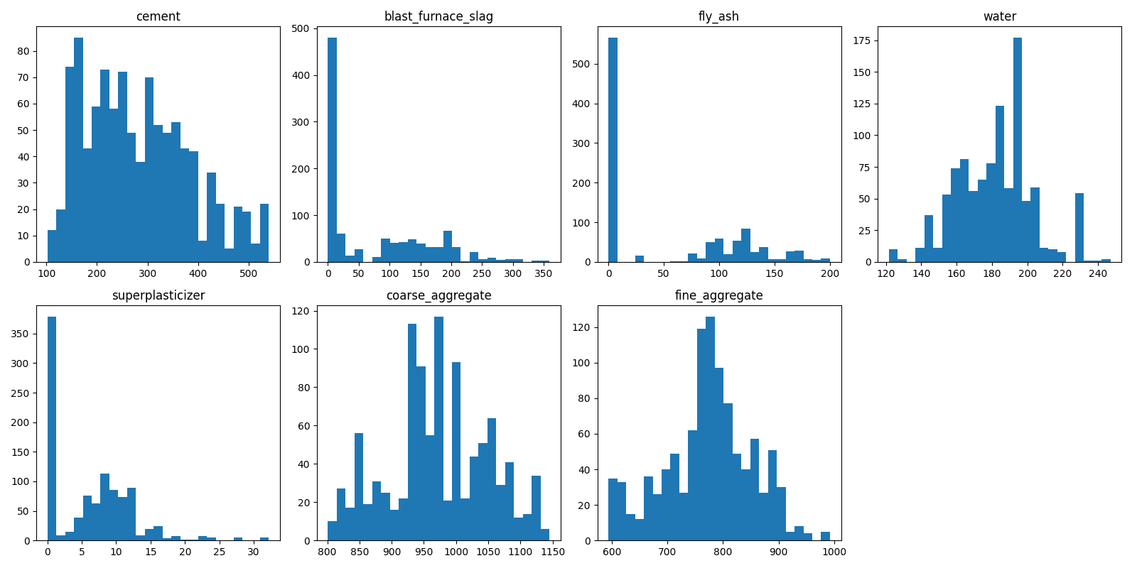
Plotting each input column (leaving out age for now) shows a mixed picture. Some columns, like cement and water, are already reasonably close to a bell shape. Others, like superplasticizer, blast_furnace_slag, and fly_ash, are clearly skewed, each with a tall spike at 0 and a long tail stretching right.
age is skewed enough that it's worth plotting on its own:
df['age'].hist(bins=30)
plt.title('age')
plt.show()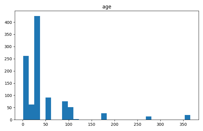
The worst offender by far is age: a lot of concrete samples are tested young, and a much smaller number are tested very old, so the column is heavily lopsided rather than bell-shaped. Its skew value backs that up, df['age'].skew() comes out to roughly 3.27, by far the largest of any column here.
Outliers were left untouched on purpose. No outlier removal was done before comparing "with transform" against "without transform". That was intentional: the goal here is to isolate the effect of the transform itself, not mix it with the effect of outlier handling.
Step 4: Apply Box-Cox
Since Box-Cox needs every value to be strictly positive, the columns with zeros (blast furnace slag, fly ash, superplasticizer) need a tiny nudge first, adding a very small constant so the zeros become just barely positive without meaningfully changing the data:
X_train['blast_furnace_slag'] = X_train['blast_furnace_slag'] + 0.001
# same small addition applied to the other zero-containing columns

from sklearn.preprocessing import PowerTransformer

pt = PowerTransformer(method='box-cox')
X_train_transformed = pt.fit_transform(X_train)
X_test_transformed = pt.transform(X_test)
Retrain on the transformed data and check a single split first:
lr.fit(X_train_transformed, y_train)
lr.score(X_test_transformed, y_test)  # single-split R2, noticeably higher than the untouched baseline
Then confirm it with cross-validation, the same way the baseline was checked in Step 2. Since PowerTransformer has to be fit fresh on each cross-validation fold, not just once on X_train, it needs to go inside a Pipeline so cross_val_score can refit it correctly on every fold:
from sklearn.pipeline import Pipeline

zero_cols = ['blast_furnace_slag', 'fly_ash', 'superplasticizer']
X_shifted = X.copy()
X_shifted[zero_cols] = X_shifted[zero_cols] + 0.001

box_cox_pipe = Pipeline([
    ('power_transform', PowerTransformer(method='box-cox')),
    ('linear_reg', LinearRegression()),
])

cross_val_score(box_cox_pipe, X_shifted, y, cv=10, scoring='r2').mean()
Retraining Linear Regression on this transformed data gives a noticeably better R2 score than the untouched baseline, both on a single split and under cross-validation. The improvement isn't dramatic, but it's consistent and real.
Step 5: Apply Yeo-Johnson
Because Yeo-Johnson doesn't care about zeros, this version skips the small-constant workaround entirely:
pt2 = PowerTransformer()  # method='yeo-johnson' is the default
X_train_transformed2 = pt2.fit_transform(X_train)
X_test_transformed2 = pt2.transform(X_test)
Retraining again on this version gives a further improvement over the Box-Cox result, at least in this example. That lines up with what you'd generally expect: Yeo-Johnson is the more flexible, more modern of the two, and it's what most recent guidance defaults to.
PowerTransformerstandardizes for you. By default,standardize=True, meaning the output isn't just reshaped, it also comes back with a mean of0and a standard deviation of1, the same thingStandardScalernormally does. You don't need to add a separate scaling step afterward.
Step 6: Inspect the Lambda Values
Every column gets fit with its own lambda, and it's worth looking at what the transform actually decided:
pt2.lambdas_array([ 0.17428121, 0.01571083, -0.16144864, 0.7725385 , 0.25361555,
1.12996936, 1.78299001, 0.0198852 ])
Lining these up against X_train.columns makes them easier to read:
pd.Series(pt2.lambdas_, index=X_train.columns)cement 0.174281
blast_furnace_slag 0.015711
fly_ash -0.161449
water 0.772538
superplasticizer 0.253616
coarse_aggregate 1.129969
fine_aggregate 1.782990
age 0.019885
dtype: float64
Each number lines up with one input column, in order. A lambda close to 1 means "barely any change was needed", while a lambda far from 1 (closer to 0, or negative) means that column needed a much stronger reshaping to look normal. That tracks with what Step 3 already showed: coarse_aggregate (1.13) and water (0.77) were already close to normal and got lambdas near 1, while age (0.02) and fly_ash (-0.16), the most visibly skewed columns, got pulled down toward the log-like end of the scale to fix that.
Step 7: Compare the Distributions Visually
X_train_t2_df = pd.DataFrame(X_train_transformed2, columns=X_train.columns)

fig, axes = plt.subplots(1, 2, figsize=(10, 4))
axes[0].hist(X_train['age'], bins=30)
axes[0].set_title('age: before')
axes[1].hist(X_train_t2_df['age'], bins=30)
axes[1].set_title('age: after Yeo-Johnson')
plt.tight_layout()
plt.show()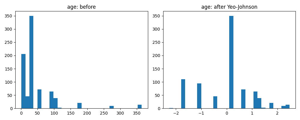
age, the worst-skewed column going in, comes out looking dramatically more like a bell curve. The long thin tail of old samples is gone, replaced by a distribution that actually spreads out on both sides of its center.
The same before/after comparison for the rest of the columns:
cols = ['cement', 'water', 'superplasticizer', 'coarse_aggregate', 'fine_aggregate']

fig, axes = plt.subplots(len(cols), 2, figsize=(9, 3 * len(cols)))
for i, col in enumerate(cols):
    axes[i, 0].hist(X_train[col], bins=25)
    axes[i, 0].set_title(f'{col}: before')
    axes[i, 1].hist(X_train_t2_df[col], bins=25)
    axes[i, 1].set_title(f'{col}: after Yeo-Johnson')
plt.tight_layout()
plt.show()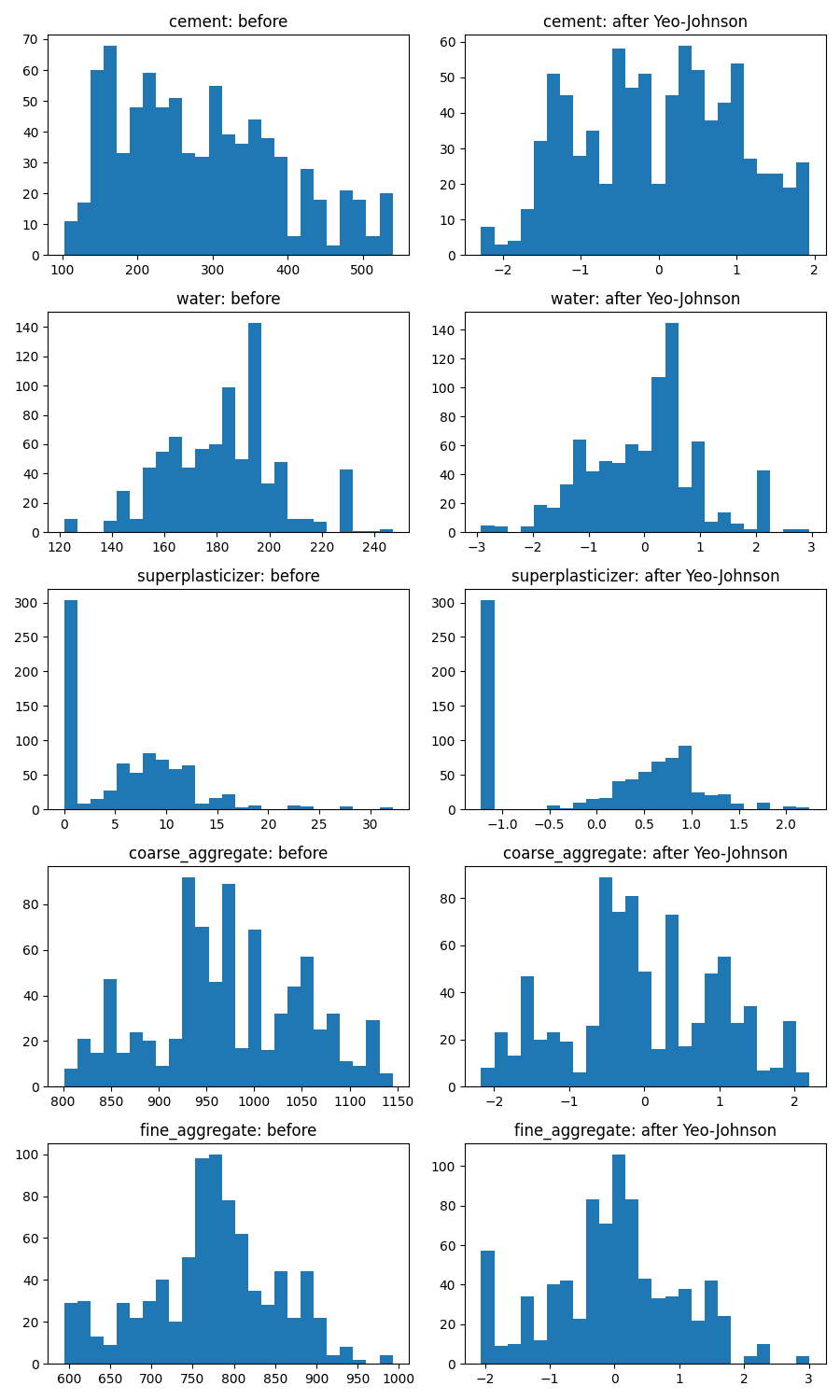
Columns that were already close to normal, like cement and water, barely change shape, which makes sense: there wasn't much left to fix, PowerTransformer mostly just rescales them. superplasticizer shows a moderate improvement: the spike of zero-valued rows is still there (a transform can't erase that many identical values), but the rest of the distribution spreads out more evenly instead of trailing off in one long tail. coarse_aggregate and fine_aggregate, which were reasonably well-behaved to begin with, stay about the same shape, just rescaled to a standardized range.
Box-Cox vs. Yeo-Johnson: Which One Should You Use?
The practical rule from this walkthrough: if every value in your column is strictly greater than zero, either technique is worth trying. If any value is zero or negative, skip straight to Yeo-Johnson rather than patching Box-Cox with workarounds. When in doubt, try both and let cross-validation tell you which one actually helped.
This isn't a replacement for trying Log or Square Root.
PowerTransformerusually performs at least as well as the simpler formulas from the last post, often a bit better, since it's tuning itself to your exact data instead of using a one-size-fits-all formula. But "usually" isn't "always". Trying bothFunctionTransformerandPowerTransformerand comparing cross-validated results is still the safest way to know which one wins on your dataset.
The Big Takeaway
PowerTransformerautomatically finds the best exponent (lambda) to reshape each column toward a normal distribution, instead of you guessing a fixed formula.- Box-Cox is the original technique, but only works on strictly positive data.
- Yeo-Johnson does the same job but also handles zero and negative values, which is why it's scikit-learn's default.
- The output is standardized automatically (mean
0, standard deviation1), so there's no need for a separate scaling step. - This only matters for statistical models like Linear and Logistic Regression. Tree-based models don't need any of this.
- Always confirm an improvement with cross-validation, not a single train/test split, before trusting that a transform actually helped.
Summary Cheat Sheet
| Property / Aspect | Detail |
|---|---|
| Used For | Automatically finding and applying the best power transform to make a column more normal |
| Import | sklearn.preprocessing.PowerTransformer |
| Two Methods | method='box-cox' and method='yeo-johnson' (default) |
| Box-Cox Restriction | Requires strictly positive values; fails on zero or negative data |
| Yeo-Johnson Advantage | Works on positive, zero, and negative values |
| How Lambda Is Chosen | Searched across a range (roughly -5 to 5) using Maximum Likelihood Estimation |
| Inspecting Lambdas | .lambdas_ attribute, one value per input column |
| Standardization | Automatic by default (standardize=True); no separate StandardScaler needed |
| Helps | Statistical models: Linear Regression, Logistic Regression |
| Doesn't Help | Tree-based models: Decision Tree, Random Forest |
| Key Best Practice | Try both Box-Cox/Yeo-Johnson and the simpler Log/Square Root transforms, verify improvement with cross-validation |
What's Next?
Ch.21 covered FunctionTransformer and the four hand-picked formulas: Log, Reciprocal, Square, and Square Root. This post covered PowerTransformer, which searches for the best exponent automatically using Box-Cox or Yeo-Johnson. Together, these close out the mathematical transformations part of this feature engineering series. Based on how this series has progressed so far, from encoding to scaling to reshaping, the next logical stop is likely Binning and Discretization: grouping a continuous numerical column into a smaller number of buckets, another common feature engineering step worth knowing before moving on to more advanced topics.