
Ch.26: Handling Missing Data with Complete Case Analysis
Inspired by: YouTube
Every feature engineering post so far has assumed the data is actually there, just in an inconvenient shape: numbers on different scales, categories as text, dates as strings. This post starts a different problem: what happens when the data simply isn't there at all. Almost every machine learning algorithm chokes on missing values, so cleaning them out (or filling them in) isn't optional, it's a required step before training. This is the first of several posts on the topic, and it covers the simplest option: Complete Case Analysis, dropping rows that have any missing data at all.
Two Ways to Handle Missing Data
When a column has missing values, there are exactly two options:
- Delete the rows (or columns) that have missing values.
- Impute the missing values, fill them in with something reasonable.
Deletion is covered in this post. Imputation splits further into univariate techniques (mean, median, random sample, or "end of distribution" for numerical columns; mode or a placeholder like "Missing" for categorical ones) and multivariate techniques (KNN Imputer, Iterative Imputer), each of which gets its own post later in this series.
What Is Complete Case Analysis?
Complete Case Analysis (CCA), also called listwise deletion, means discarding every row that has a missing value in any column, and keeping only the rows where every single column is filled in. Picture a dataset with four columns, three inputs and one output, and five rows. If the third row is missing a value in the first column, CCA removes that entire row, leaving four complete rows to work with. It's called "complete case" because only cases (rows) with complete information across every column survive.
Advantages
- Trivial to implement. One line,
df.dropna(), and there's no data manipulation logic to get wrong. - Preserves the distribution of the remaining columns, as long as the assumption below holds.
Disadvantages
- It can throw away a large fraction of the dataset. If several columns each have some missing data, the rows lost to any one of them all stack up, and a wide dataset can shrink fast.
- It distorts the distribution if the data isn't missing randomly. This is the disadvantage that matters most, and it's covered next.
- A production model won't know how to handle missing values. If a model is trained only on rows that happened to have zero missing data, it has never seen a missing value during training. The moment real-world input arrives with a gap in it, the model has no learned strategy for it. This is exactly why CCA isn't used as heavily as its simplicity would suggest.
The MCAR Assumption
CCA is only safe when data is Missing Completely At Random (MCAR), meaning the fact that a value is missing has nothing to do with any other value in the dataset, the missingness itself is pure noise. If 50 values are missing out of 1,000 rows, MCAR means those 50 could be scattered anywhere: the first 50 rows, the last 50, or spread evenly, it makes no difference, because there's no underlying pattern connecting which rows lost data to anything else in the dataset.
Why this matters: if missingness actually correlates with something else in the data (say, a column is more often missing for one particular category), then dropping those rows doesn't just remove random noise, it systematically removes a subset of the population. The distribution of the remaining columns shifts, and any model trained on what's left has learned a biased picture.
The practical rule: apply CCA only when both of these hold.
- The data is MCAR. There's no way to prove this with certainty, but it can be checked, and the next section shows how.
- Less than 5% of a column is missing. There's no strict law behind this number, it's a widely used convention. Under 5%, the rows lost are a small enough slice that even in the worst case, the damage is limited. Over that, CCA starts trading away too much of the dataset. If a column has extreme missingness, like 95%+, the better move isn't CCA on the rows, it's dropping the column entirely, since it carries almost no usable signal anyway.
Trying It on a Real Dataset
This dataset tracks candidates who applied for data science jobs, one row per applicant, columns describing their city, education, experience, current company, and whether they were ultimately hired (target).
import pandas as pd

df = pd.read_csv('data_science_job.csv')
df.shape
(19158, 13)Step One: Check What's Missing
df.isnull().mean() * 100enrollee_id 0.00
city 0.00
city_development_index 2.50
gender 23.53
relevent_experience 0.00
enrolled_university 2.01
education_level 2.40
major_discipline 14.68
experience 0.34
company_size 30.99
company_type 32.05
training_hours 4.00
target 0.00
dtype: float64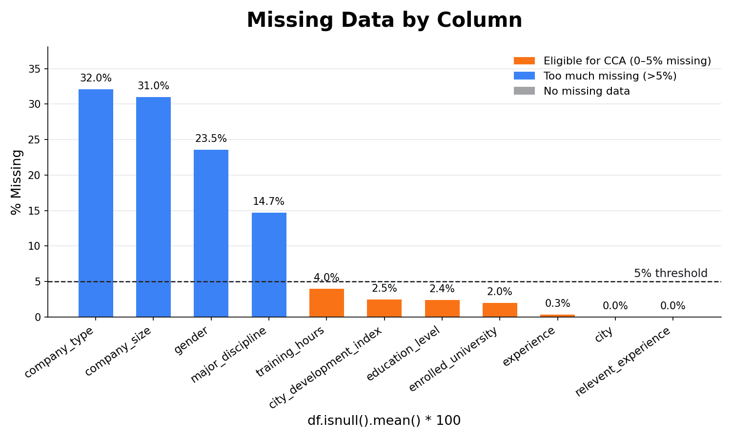
Four columns are well past the 5% line: company_type (32%), company_size (31%), gender (23.5%), and major_discipline (14.7%). CCA on any of those would mean losing a fifth to a third of the entire dataset, and that's before accounting for whatever other columns are also missing in the surviving rows. Those columns are not CCA candidates.
Five columns sit comfortably under 5%: training_hours (4.0%), city_development_index (2.5%), education_level (2.4%), enrolled_university (2.0%), and experience (0.3%). Those five are what this post applies CCA to, picked out with a list comprehension instead of typing the names by hand, so the same line still works if the dataset's columns change:
cols = [col for col in df.columns if 0 < df[col].isnull().mean() < 0.05]
cols
['city_development_index', 'enrolled_university', 'education_level',
'experience', 'training_hours']new_df = df[cols].dropna()Step Two: Check How Much Data Survives
len(new_df) / len(df)0.8969...Roughly 90% of the rows survive, 17,182 out of 19,158. That's the first sanity check: not so much data lost that the exercise is pointless.
Step Three: Compare Distributions Before and After
Row count surviving isn't enough on its own, the shape of what's left matters just as much. If dropping rows shifted the distributions, that's a signal the data wasn't MCAR after all.
For a numerical column like training_hours, that means comparing histograms before and after:
import matplotlib.pyplot as plt

fig, ax = plt.subplots()
df['training_hours'].hist(bins=40, density=True, alpha=0.5, label='Original', ax=ax)
new_df['training_hours'].hist(bins=40, density=True, alpha=0.5, label='After CCA', ax=ax)
ax.legend()
plt.show()
For a categorical column like education_level, the equivalent check is comparing the proportion each category makes up before and after:
df['education_level'].value_counts(normalize=True)
new_df['education_level'].value_counts(normalize=True)
Graduate 0.620
Masters 0.233
High School 0.108
Phd 0.022
Primary School 0.016Graduate 0.620
Masters 0.234
High School 0.107
Phd 0.022
Primary School 0.017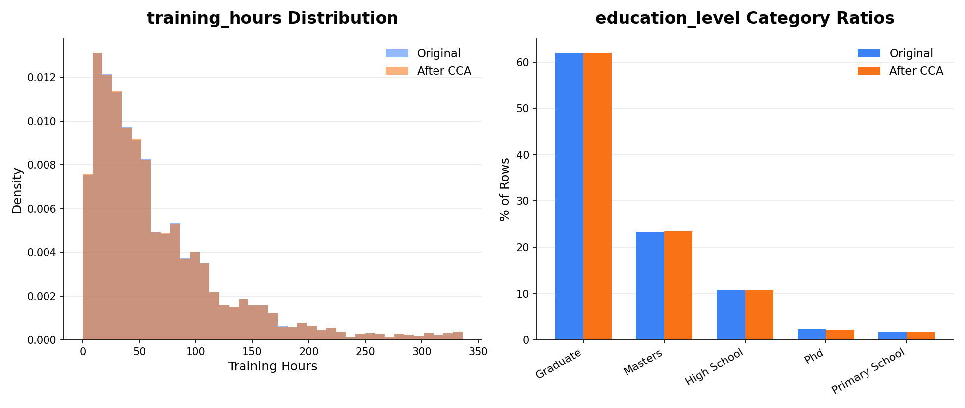
Both checks agree. The training_hours histogram overlaps itself almost perfectly, blue (original) and orange (after CCA) barely diverge anywhere along the range. The education_level proportions move by less than half a percentage point in every category, Graduate stays at 62.0%, Masters goes from 23.3% to 23.4%, and so on. Neither shows the kind of shift that would suggest the missing values were tied to any particular group. That's the evidence needed to call this data MCAR, and it's what makes CCA a reasonable choice here.
If instead one category's share had jumped by several points, say Masters moved from 19% to 25%, that would be a red flag: it would mean masters-level candidates were disproportionately represented among the complete rows, which means the missing values in some other column weren't random with respect to education level. In that situation, CCA would be actively harmful, dropping rows wouldn't just shrink the dataset, it would skew it, and the fix would be to fall back on imputation instead.
Summary Cheat Sheet
| Task | Code |
|---|---|
| Check % missing per column | df.isnull().mean() * 100 |
| Apply CCA on chosen columns | df[cols].dropna() |
| Check rows retained | len(new_df) / len(df) |
| Compare numerical distributions | overlaid .hist() before vs. after |
| Compare categorical ratios | .value_counts(normalize=True) before vs. after |
| When to apply CCA | data is MCAR, and column has < 5% missing |
What's Next?
This post covered the simplest way to handle missing data: dropping rows entirely with Complete Case Analysis, and how to check whether that's actually a safe move (the MCAR assumption, the 5% rule, and comparing distributions before and after). It's rarely used in production because a model trained this way never learns to handle missing values it will inevitably see later. The next posts in this series move to the more common approach: imputation, starting with univariate techniques using scikit-learn's SimpleImputer.