Ch.1: Simple Linear Regression - The Intuition

Inspired by: YouTube

This starts a new series that goes through machine learning algorithms one at a time, in depth. The first one almost everyone learns is linear regression. It's not the most powerful algorithm out there, support vector machines or ensemble methods will usually beat it on raw accuracy, but it's the most primitive and easy to understand, which makes it the right place to build intuition before things get more complex.

The Landscape

Linear regression sits under supervised learning, and specifically it solves regression problems: predicting a continuous numeric value rather than a category. Within linear regression itself there are three variants worth knowing about upfront:

• Simple linear regression: one input column, one output column.
• Multiple linear regression: more than one input column.
• Regularized regression (Ridge, Lasso, and friends): variants that constrain the model to avoid overfitting.

This post focuses entirely on simple linear regression. Once that's solid, multiple linear regression is a small extension, not a new idea.

The Dataset

The example dataset is a college placement record: 200 students, two columns, cgpa and package (their salary in LPA, lakhs per annum). The goal is to build a model that, given a new student's CGPA, predicts what package they're likely to get.

import pandas as pd
 
df = pd.read_csv('placement.csv')
df.head()

   cgpa  package
0  6.89     3.26
1  5.12     1.98
2  7.82     3.25
3  7.42     3.67
4  6.94     3.57

Plotting cgpa against package makes the shape of the problem obvious:

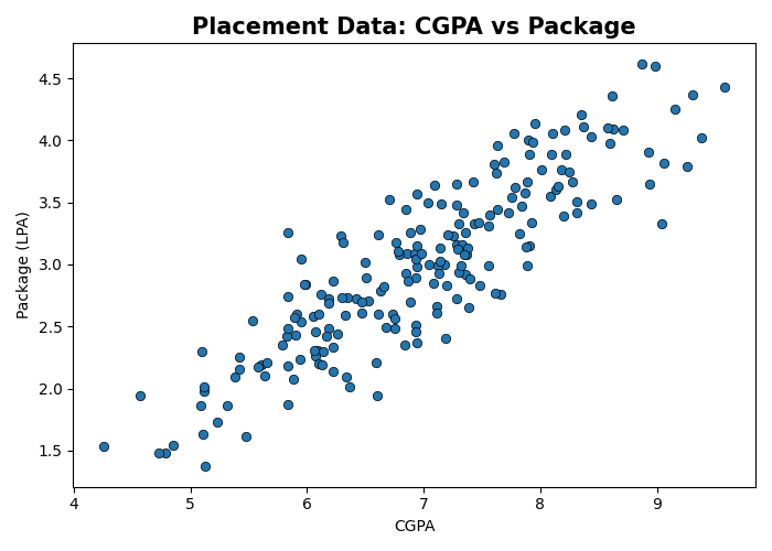
The trend is clearly upward and roughly linear, but it's not a perfect line. That's expected: real-world data is noisy. A student with a CGPA of 7.2 might land a package of 4.5 LPA while another student with the exact same CGPA lands 2.8 LPA. Interview performance, the specific company, negotiation, luck, none of that is captured in a CGPA number, so the same input can map to different outputs. This isn't a flaw in the data, it's just how real data behaves.

Fitting the Best Fit Line

Since the data isn't perfectly linear, the goal shifts from "find the line that passes through every point" to "find the line that minimizes overall error." That line is called the best fit line, and it's what linear regression is actually searching for.

X = df.iloc[:, 0:1]
y = df.iloc[:, -1]
 
from sklearn.model_selection import train_test_split
X_train, X_test, y_train, y_test = train_test_split(X, y, test_size=0.2, random_state=2)
 
from sklearn.linear_model import LinearRegression
lr = LinearRegression()
lr.fit(X_train, y_train)

That's it. Training a linear regression model in sklearn is three lines once the data is split. Now check a prediction against reality:

lr.predict(X_test.iloc[0].values.reshape(1, 1))

The first test student has a CGPA of 8.58 and an actual package of 4.10 LPA. The model predicts:

array([3.89])

Not exact, but close, which is the point. Plotting the fitted line over the data shows what "best fit" looks like geometrically:

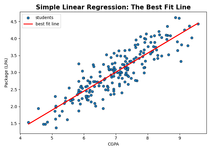
The red line doesn't touch most of the points. It doesn't need to. It's the line that makes the smallest total error across all 200 students, which is a very different goal from passing through every point exactly.

What the Line Actually Is

Under the hood, sklearn found the equation of a straight line: y = mx + b. Both values are sitting on the fitted model:

m = lr.coef_
b = lr.intercept_

m = 0.5580
b = -0.8961

With those two numbers, predicting for any CGPA is just arithmetic:

m * 8.58 + b   # 3.89
m * 9.5 + b    # 4.40

What Slope and Intercept Actually Mean

m and b aren't just numbers a solver spat out, they carry meaning.

m, the slope, is how much the output depends on the input. A small slope means package barely moves as CGPA changes. A large slope means small CGPA changes swing the predicted package a lot. It's effectively a weight: how much this one input column matters to the prediction.

b, the intercept, is what the model predicts when the input is zero. Left alone, that's often a nonsensical number, plug cgpa = 0 into this model and it would predict a negative package, which doesn't make real-world sense. b isn't trying to be a real prediction at zero; it's a correction term. It's what keeps the line anchored correctly even when the input's meaningful range never actually reaches zero. Without it, every line would be forced to pass through the origin, which is far too rigid a constraint for real data.

Where This Breaks

The line is only ever a model of the data it was trained on, not a law of nature. Push the input far outside the range it was trained on and the predictions stop making sense:

m * 100 + b

54.9

A CGPA of 100 predicting a package of 54.9 LPA is obviously absurd, CGPA doesn't even go past 10. The model has no concept of "this input is nonsense", it just keeps applying the same straight-line formula forever in both directions. That's a good reminder to keep in mind for every algorithm in this series: a model is only as trustworthy as the range of data it was actually trained on.

What's Next

This post covered the geometric intuition: linear regression draws a best fit line, and slope and intercept each carry a distinct meaning. The next post works out the actual math behind how m and b get calculated, deriving the closed-form OLS solution by hand and then coding a linear regression class from scratch to compare against sklearn's version.