
Ch.9: Stochastic Gradient Descent
Inspired by: YouTube
The previous post implemented GDRegressor, a batch gradient descent class that trains on the full 353-row diabetes dataset and hits test R² = 0.4535 in 1000 epochs. Before moving on, it is worth asking: what happens when the dataset has 1 million rows instead of 353? Or 100,000 features? The batch GD loop does not scale to either case, and understanding exactly why motivates every variant of gradient descent that follows.
The Scaling Problem with Batch GD
Recall the batch GD update rule for a single coefficient :
The key word is : every derivative you compute requires visiting all rows. For rows and features (so parameters), and 15 epochs, you compute approximately derivative terms per training run. Push that to rows, features, and epochs, and the total is derivative terms. That is a lot of computation for one model fit, and it compounds as the model gets deeper or wider.
There is a second, more fundamental problem: memory. The vectorized batch GD update, y_hat = X_train @ coef_ + intercept_, requires the entire X_train matrix to be resident in RAM at the same time. For a dataset with rows and float64 columns, X_train alone occupies roughly MB. Larger datasets do not fit at all, or they do but leave no headroom for the model, gradients, or anything else. When the system runs out of memory, the computation fails entirely. This is not a solvable problem by buying a faster CPU; it is a structural limitation of the algorithm.
These two problems are distinct:
- Computational cost: too many multiply-accumulate operations per epoch.
- Memory cost: must load all of
X_traininto RAM before a single update can happen.
Stochastic Gradient Descent solves both.
The SGD Idea: One Row at a Time
The insight behind SGD is simple: you do not need the exact gradient to make progress. You need a gradient that, on average over many steps, points in the right direction. A single randomly selected row gives you a noisy but unbiased estimate of the true gradient.
Instead of one update per epoch using all rows:
SGD takes updates per epoch, one per row, using only that row's gradient:
where row is chosen randomly each time. The randomness is not incidental; it is the defining characteristic of the algorithm (the word "stochastic" comes from the Greek for "random" or "probabilistic").
What Changes in the Derivative
For a single row , the prediction is just one number:
The loss for that single row is the squared error . Differentiating with respect to and :
Compare these to the batch GD derivatives. The batch version sums over all rows and divides by (taking a mean). The SGD version has no sum, no mean, no division. It is just times the residual for that single row, times the feature value for the intercept or coefficient respectively. Because there is only one row, the summation collapses to a single term, and averaging it would just divide by 1.
This is the only mathematical difference between batch GD and SGD. The update rule structure is identical; only the scope of the gradient estimate changes.
Implementing SGDRegressor from Scratch
The implementation follows the source notebook in day52-types-of-gradient-descent. The class structure mirrors GDRegressor from the previous post exactly; the only changes are inside the fit loop.
The Dataset (Same as Ch.8)
from sklearn.datasets import load_diabetes
import numpy as np
from sklearn.linear_model import LinearRegression
from sklearn.metrics import r2_score
from sklearn.model_selection import train_test_split

X, y = load_diabetes(return_X_y=True)
X_train, X_test, y_train, y_test = train_test_split(
    X, y, test_size=0.2, random_state=2
)
print(X_train.shape)  # (353, 10)
Same split, same random_state=2, so our results are directly comparable to Ch.8.
The SGDRegressor Class
class SGDRegressor:
    def __init__(self, learning_rate=0.01, epochs=1000):
        self.lr = learning_rate
        self.epochs = epochs
        self.coef_ = None
        self.intercept_ = None

    def fit(self, X_train, y_train):
        # Initialize exactly like GDRegressor
        self.intercept_ = 0
        self.coef_ = np.ones(X_train.shape[1])

        for i in range(self.epochs):
            for j in range(X_train.shape[0]):
                # Pick one row at random
                idx = np.random.randint(0, X_train.shape[0])

                # Prediction for that single row
                y_hat = np.dot(X_train[idx], self.coef_) + self.intercept_

                # Intercept gradient: -2 * residual (no mean, single sample)
                intercept_der = -2 * (y_train[idx] - y_hat)
                self.intercept_ -= self.lr * intercept_der

                # Coefficient gradient: -2 * residual * feature_row (no mean)
                coef_der = -2 * (y_train[idx] - y_hat) * X_train[idx]
                self.coef_ -= self.lr * coef_der

    def predict(self, X):
        return X @ self.coef_ + self.intercept_
A few design points worth noting carefully:
The inner loop runs X_train.shape[0] times per epoch. Each iteration picks one random index and does one parameter update. So in a single epoch, the model updates its parameters 353 times (once per row in the training set). Batch GD updates once per epoch. This means one epoch of SGD involves 353 times more parameter updates than one epoch of batch GD.
np.random.randint(0, X_train.shape[0]) samples uniformly from [0, n) with replacement. It is not shuffling and iterating in order; it is genuinely random each time. The same row index can be picked multiple times in the same epoch, and some rows might not be picked at all. This is intentional: it is the stochastic part.
np.dot(X_train[idx], self.coef_) takes one row of X_train (shape (10,)) and dots it with the coefficient vector (shape (10,)), producing a single scalar prediction. There is no matrix multiply, no broadcasting; just one dot product per update. This is what avoids the memory problem: you only ever need one row in memory at a time, not the full X_train.
The intercept update uses the raw residual, not its mean: intercept_der = -2 * (y_train[idx] - y_hat). In batch GD, the factor was -2 * np.mean(residuals). Here it is just -2 * scalar_residual. Both are valid gradient estimates for their respective loss functions. The learning rate absorbs the scaling difference.
Running and Evaluating
np.random.seed(42)
sgd = SGDRegressor(learning_rate=0.01, epochs=1000)
sgd.fit(X_train, y_train)

print("SGD intercept:", sgd.intercept_)
# 151.81000

print("SGD coef_:", sgd.coef_)
# [ -12.14, -206.12,  533.12,  342.29, -137.17,
#    -52.58, -169.54,   53.98,  578.12,   47.66]

y_pred_sgd = sgd.predict(X_test)
print("SGD R2:", r2_score(y_test, y_pred_sgd))
# 0.4424| Model | Test R² |
|---|---|
| sklearn OLS (Ch.8) | 0.4399 |
| Batch GDRegressor (Ch.8) | 0.4535 |
| SGDRegressor (this post) | 0.4424 |
SGD lands between OLS and batch GD on this dataset. The intercept (151.81) is very close to OLS (151.88), confirming the model found roughly the right mean offset. The notable divergence is on through , the six serum measurements: SGD lands at for vs OLS's , and for vs OLS's . These features are highly correlated with each other, so the loss surface along their directions is very flat, and both the random row selection and the noisier gradient path mean SGD arrives at a different point on the same nearly-flat ridge than either OLS or batch GD.
Running the exact same code again with a different seed will give you slightly different numbers. That is expected, not a bug.
The Noisy Path to Convergence
The convergence behavior of SGD is fundamentally different from batch GD, and it is visible in the chart below.
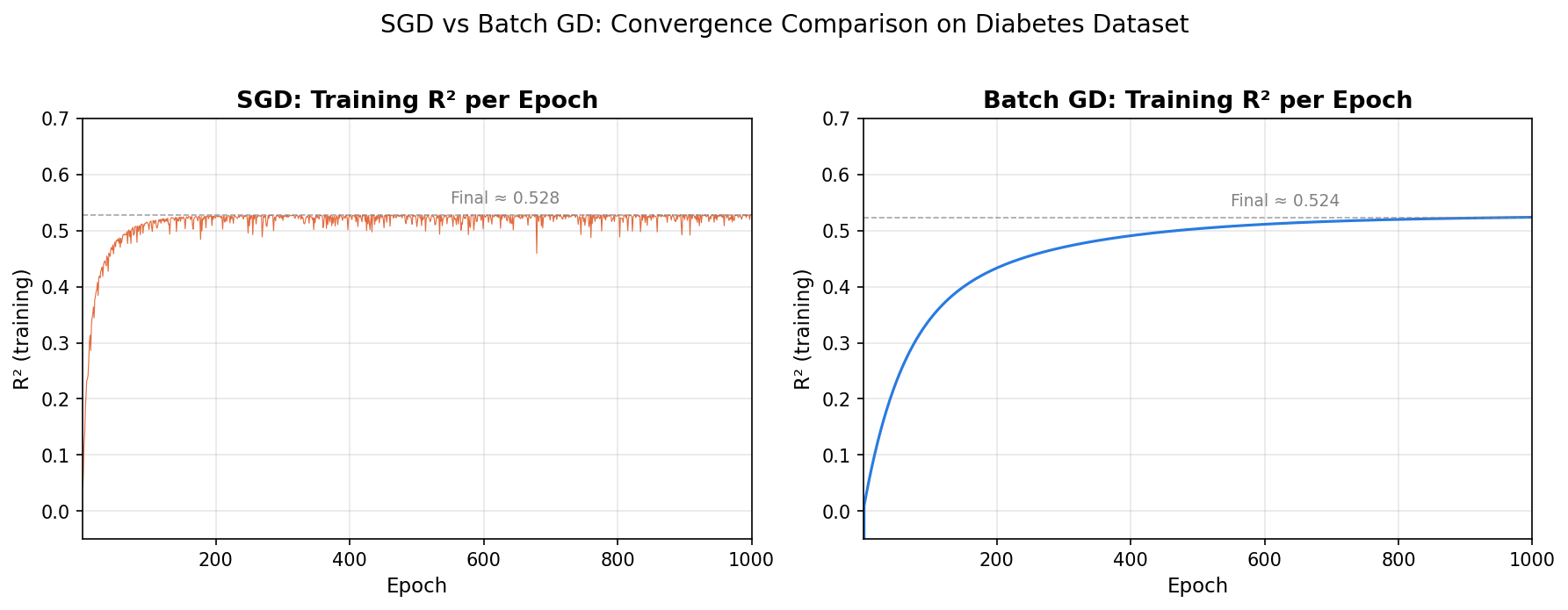
Left (SGD): The training R² shoots up from 0 to about 0.50 within the first 50 epochs, then oscillates around 0.53 for the remaining 950 epochs. The curve never settles. Every epoch introduces new randomness (a different sequence of 353 randomly chosen rows), so the gradient estimates are always noisy. After roughly 100 epochs, SGD has essentially found the neighborhood of the optimum, but it cannot converge to a single fixed point because there is no mechanism to quiet the noise as you approach it.
Right (Batch GD): The curve rises smoothly and monotonically. Each epoch uses the same full-dataset gradient, which points precisely toward the optimum. The curve is still not flat at epoch 1000 (there is more improvement available with more epochs), but it does not oscillate at all. Every step is guaranteed to improve or maintain the loss.
The key observation: SGD reaches a good region much faster in epoch count, but it never truly "converges" in the way batch GD does. It oscillates around the optimum permanently. This is a fundamental property of the algorithm, not a bug to be fixed with more epochs.
There is a practical fix called a learning schedule (or learning rate decay): decrease the learning rate as training progresses. At a high learning rate, the large random steps help you find the right neighborhood quickly. As you reduce the learning rate, the step sizes shrink and the oscillation tightens. At a very small learning rate, SGD behaves more like batch GD in a small region around the optimum. In scikit-learn's SGDRegressor, the learning_rate parameter ('constant', 'optimal', 'invscaling', or 'adaptive') controls this behavior directly.
Wall-Clock Time: The Counterintuitive Result
import time

# Batch GD: 1000 epochs
start = time.time()
gd = GDRegressor(learning_rate=0.5, epochs=1000)
gd.fit(X_train, y_train)
print(f"Batch GD time: {time.time() - start:.4f}s")
# Batch GD time: 0.0172s

# SGD: same 1000 epochs
np.random.seed(42)
start = time.time()
sgd = SGDRegressor(learning_rate=0.01, epochs=1000)
sgd.fit(X_train, y_train)
print(f"SGD time: {time.time() - start:.4f}s")
# SGD time: 1.9050s
This surprises many people. SGD is supposed to be faster, but here it took about 110 times longer for the same number of epochs. How?
The answer is in the update count. At rows and 1000 epochs:
| Algorithm | Updates per epoch | Total updates |
|---|---|---|
| Batch GD | 1 | 1,000 |
| SGD | 353 | 353,000 |
SGD does 353,000 parameter updates to batch GD's 1,000. Each update involves a Python loop iteration, a random index draw, a dot product, two gradient computations, and two in-place subtractions. Batch GD does all of that in one vectorized NumPy call per epoch. On a small dataset like this, NumPy's vectorized matrix operations are so fast that the pure Python overhead of 353,000 serial iterations dwarfs any per-epoch savings.
This is not a flaw in SGD. It is a dataset-size mismatch. The efficiency argument for SGD is not that it is faster per update; it is that it needs far fewer epochs to reach a good solution. On this 353-row dataset, batch GD converges quickly too, so the epoch count advantage of SGD never materializes. On a dataset with 10 million rows:
- Batch GD cannot even start:
X_trainis multiple GB, and one matrix multiply per epoch requires the entire thing in RAM. - SGD looks at one row per update, needs trivial memory, and reaches a useful model in far fewer total sweeps of the data.
The real speed advantage of SGD only becomes visible when batch GD is struggling. On huge datasets, batch GD's overhead is not just slower; it is impossible. SGD is the algorithm that makes large-scale machine learning tractable.
When to Use SGD
Two cases where SGD is clearly superior to batch GD:
1. Big data. When the dataset is large enough that loading all of X_train at once would exhaust RAM, batch GD cannot run at all. SGD only needs one row at a time. Its training-set memory footprint is per update (one row of features) rather than for the whole matrix.
2. Non-convex loss functions. Linear regression has a convex squared-error loss, so batch GD always finds the global minimum. Logistic regression, neural networks, and SVMs can have non-convex losses with multiple local minima. Batch GD, because it follows the gradient smoothly and monotonically, can get trapped in a local minimum and never escape. SGD's random noise acts like a perturbation: when the gradient estimate from a particular row points in an unusual direction, it can kick the parameters out of a shallow local minimum. The jagged convergence path that looks like a disadvantage on a convex problem is actually what allows SGD to escape local optima on non-convex ones. You need to tune the learning rate carefully to exploit this, but it is one reason SGD and its mini-batch variant are the standard optimizer for neural networks.
Sklearn's SGDRegressor
For completeness, the transcript also demonstrates sklearn's built-in version:
from sklearn.linear_model import SGDRegressor as SklearnSGD

sk_sgd = SklearnSGD(max_iter=100, learning_rate='constant', eta0=0.01)
sk_sgd.fit(X_train, y_train)
y_pred_sk = sk_sgd.predict(X_test)
print("sklearn SGD R2:", r2_score(y_test, y_pred_sk))
Sklearn's version supports multiple loss functions (not just squared error), regularization (L1, L2, ElasticNet via the penalty parameter), adaptive learning rate schedules, and early stopping via a tol parameter. It is the class you would use in production; our SGDRegressor above is the class you would use to understand what it is actually doing internally.
Summary & Key Takeaways
- Why batch GD doesn't scale: computing the gradient requires visiting all rows and holding the full
X_trainin RAM simultaneously. For large or large feature count , this becomes computationally and memory-prohibitive. - SGD's core idea: replace the full-dataset gradient with a gradient computed from a single randomly chosen row. Update parameters immediately, before looking at the next row.
- The derivative simplification: with one row, the summation collapses to a single term; no mean is needed. The intercept gradient is ; the coefficient gradient is .
- Memory efficiency: each update uses only one row of data. The memory footprint per update is rather than , so datasets too large for RAM become trainable.
- More updates per epoch: SGD takes parameter updates per epoch versus 1 for batch GD. Fewer epochs are needed to reach a good region of parameter space, which is the source of SGD's epoch-count advantage.
- No convergence to a fixed point: because each gradient estimate is random, SGD oscillates around the optimum permanently rather than settling. The solution varies slightly each time you run it.
- The wall-clock time paradox: on a small dataset like diabetes (353 rows), SGD is much slower per unit of time because its 353,000 Python-loop updates outpace any per-epoch savings. SGD's speed advantage only materializes on large datasets where batch GD cannot fit in memory at all.
- Non-convex advantage: SGD's noise can kick parameters out of local minima, making it the algorithm of choice for deep learning where non-convex loss surfaces are the norm.
- Learning schedules: reducing the learning rate over time narrows the oscillation band as training progresses, effectively turning SGD into a progressively finer search near the optimum. Sklearn's
SGDRegressoroffers'constant','optimal','invscaling', and'adaptive'schedules for this purpose.
In the next post, we cover Mini-Batch Gradient Descent: a middle ground between batch GD (one update per epoch over all rows) and SGD (one update per row). Mini-batch GD splits the data into small batches of rows, computes the gradient over each batch, and updates once per batch. It captures most of SGD's memory and convergence-speed benefits while using NumPy vectorization over the mini-batch to reduce Python loop overhead significantly.