Ch.53: How Feature Importance Is Actually Calculated

By Ayush Arora•2026-09-25•8 min read

Inspired by: YouTube

Every tree-based algorithm covered so far, decision trees, bagging, random forest, and the boosting methods still to come, can tell you which columns it actually relied on. This post covers what that number means, why it's useful for more than trimming columns, and, the part most tutorials skip, exactly how it's computed under the hood.

The code below follows the how-feature-importance-is-calculated.ipynb and feature-importance-in-sklearn.ipynb notebooks from the course's repo. The pixel-importance demo substitutes scikit-learn's built-in load_digits dataset (1,797 images, 8x8 pixels) for the video's full Kaggle MNIST CSV, the same idea (each pixel is a column, the model tells you which pixels matter) on a dataset small enough to actually ship in this post.

1. What Feature Importance Is, and Why It's Not Just for Feature Selection

Feature importance assigns every column a number saying how much that particular algorithm relied on it. The obvious use is feature selection: drop the low-importance columns, keep the high-importance ones, train a smaller, faster model.

The less obvious use is interpretability. If a model denies someone a loan, "the model said no" isn't an acceptable answer, the client wants to know why. If the model can also report that income and credit_history were the two highest-importance features in the decision, that's an actual explanation you can give back, not just a verdict.

2. Seeing It Visually First: Which Pixels Matter for a Digit

Before the math, a picture. Treat each pixel of a handwritten-digit image as a column, a 8x8 image is a 64-column row, and train a random forest to classify digits:

from sklearn.datasets import load_digits
from sklearn.ensemble import RandomForestClassifier
 
digits = load_digits()
X, y = digits.data, digits.target
 
rf = RandomForestClassifier(random_state=0)
rf.fit(X, y)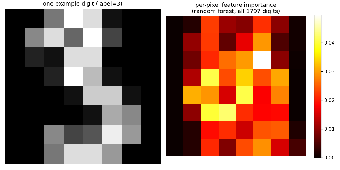

Two side-by-side images. Left, a single handwritten digit 3 rendered as an 8x8 grayscale grid. Right, a heatmap of that random forest's per-pixel feature importance, also 8x8, with the brightest yellow cells clustered in the vertical center of the grid and the darkest, near-zero cells confined to the corners and edges

rf.feature_importances_ has one value per pixel; reshaping it back into an 8x8 grid and plotting it as a heatmap shows exactly which pixels the forest actually leaned on. The corners are consistently dark, near-zero importance, because a handwritten digit almost never touches the corners of its bounding box regardless of which digit it is, so those pixels carry no information about the label. The brightest cells cluster in the vertical center, where strokes distinguishing one digit from another actually happen. This matches the intuition directly: pixels that vary a lot between different digits are useful, pixels that are almost always the same (background) are not.

3. The Formula

feature_importances_ on a fitted DecisionTreeClassifier or RandomForestClassifier is not a black box, it's a fixed, two-step formula. First, every internal node in a tree gets a node importance:

n_i = \frac{N_t}{N} \left[\text{impurity} - \left(\frac{N_{t_R}}{N_t} \times \text{right\_impurity}\right) - \left(\frac{N_{t_L}}{N_t} \times \text{left\_impurity}\right)\right]

Where $N$ is the total number of rows in the training data, $N_t$ is the number of rows that reached this specific node, and impurity (Gini or entropy) is measured before and after the split, at the node itself and at its two children. In words: node importance is the node's share of the data, times how much impurity that node's split actually removed.

Then, a column's feature importance sums the node importances of every node that split on that column, divided by the sum of every node importance in the tree:

fi_k = \frac{\sum_{j \in \text{nodes split on feature } k} n_j}{\sum_{j \in \text{all nodes}} n_j}

A column that appears at nodes covering a lot of data and removing a lot of impurity gets a high score. A column that's never split on, or only splits a handful of rows with little impurity reduction, gets a low one. The denominator normalizes everything to sum to 1 across all columns, which is why scikit-learn's docs describe the result as normalized.

4. Working It by Hand on a Real Tree

make_classification(n_samples=5, n_features=2, random_state=0) builds a tiny 5-row, 2-column dataset, small enough to compute every node importance by hand:

from sklearn.datasets import make_classification
from sklearn.tree import DecisionTreeClassifier
 
X, y = make_classification(n_samples=5, n_classes=2, n_features=2,
                            n_informative=2, n_redundant=0, random_state=0)
clf = DecisionTreeClassifier(random_state=0)
clf.fit(X, y)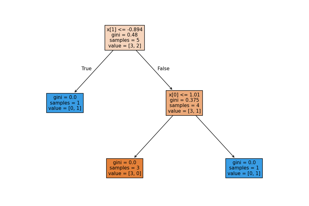

A decision tree plot with a root node splitting on x[1] <= -0.894 (gini=0.48, samples=5, value=[3, 2]), a True branch to a pure leaf (gini=0, samples=1, value=[0, 1]), and a False branch to a second internal node splitting on x[0] <= 1.01 (gini=0.375, samples=4, value=[3, 1]), which splits into two pure leaves (gini=0, samples=3, value=[3, 0] and gini=0, samples=1, value=[0, 1])

Two internal nodes, one per column. For the root (splits on x[1], the second column): $N_t = 5$ , $N = 5$ , impurity $= 0.48$ . Its right child has 4 samples and impurity 0.375; its left child has 1 sample and impurity 0 (pure).

n_{\text{root}} = \frac{5}{5}\left[0.48 - \left(\frac{4}{5} \times 0.375\right) - \left(\frac{1}{5} \times 0\right)\right] = 0.48 - 0.30 = 0.18

For the second node (splits on x[0]): $N_t = 4$ , $N = 5$ , impurity $= 0.375$ , and both its children are pure (impurity 0), so both correction terms vanish:

n_{\text{2nd node}} = \frac{4}{5}\left[0.375 - 0 - 0\right] = 0.30

Feature importance is each column's node-importance sum over the total:

fi_{x[1]} = \frac{0.18}{0.18 + 0.30} = 0.375 \qquad fi_{x[0]} = \frac{0.30}{0.18 + 0.30} = 0.625

clf.feature_importances_
# array([0.625, 0.375])

Matches exactly: x[0] (index 0) at 0.625, x[1] (index 1) at 0.375. The by-hand numbers and scikit-learn's built-in attribute agree, because they're computing the identical formula.

5. A Larger Tree, Same Method

The same formula scales to a tree with more internal nodes. make_classification(n_samples=15, ...) with the same seed produces a slightly deeper tree:

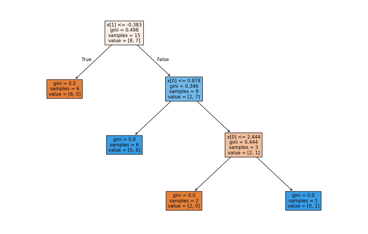
A decision tree plot with a root node splitting on x[1] <= -0.383 (samples=15), a True branch to a pure leaf (samples=6), and a False branch to a node splitting on x[0] <= 0.878 (samples=9), which leads to a pure leaf (samples=6) on one side and a third node splitting on x[0] <= 2.444 (samples=3) on the other, itself resolving into two pure leaves

Working through the same node-importance formula at each of the three internal nodes and summing by column gives:

clf.feature_importances_
# array([0.41666667, 0.58333333])

x[0] at about 0.42, x[1] at about 0.58, x[1] wins here because its single root-level split, covering all 15 rows, removes more total impurity than the two smaller x[0] splits further down combined. More nodes on a column doesn't automatically mean higher importance, what matters is how many rows each of those nodes covers and how much impurity each one actually removes.

6. Random Forest: Just an Average of the Trees' Own Importances

Random forest doesn't compute feature importance any differently, each tree computes its own feature_importances_ exactly as above, and the forest's reported importance is the plain average across all trees:

from sklearn.ensemble import RandomForestClassifier
 
rf = RandomForestClassifier(n_estimators=2, random_state=0)
rf.fit(X, y)
 
print(rf.estimators_[0].feature_importances_)  # tree 0's own importances
print(rf.estimators_[1].feature_importances_)  # tree 1's own importances
print(rf.feature_importances_)                 # the average of the two

Because each tree in the forest trains on a different bootstrap sample and column subset (Ch.48, Ch.50), its two trees can disagree sharply on which column mattered, in this run one tree came out [1.0, 0.0] and the other [0.0, 1.0], an extreme disagreement from only having 2 trees on 5 rows, averaging to [0.5, 0.5]. With hundreds of trees on a real dataset those per-tree swings cancel out into a stable, meaningful average, the same variance-reduction argument from Ch.49 applies here too, just applied to importance scores instead of predictions.

7. One Caveat: High-Cardinality Columns

scikit-learn's own documentation flags a real limitation: impurity-based feature importance, the method covered in this entire post, can be misleading for high-cardinality features, columns with many unique values (a customer ID, a raw timestamp). Such columns tend to look artificially important because a tree can use their many distinct values to carve out splits that fit the training data well without necessarily reflecting genuine predictive signal. For data with that shape, scikit-learn's permutation_importance is the documented, more reliable alternative; for ordinary columns without high cardinality, the method in this post is the standard, direct approach.

8. What to Take Away

Feature importance has two uses: trimming columns (feature selection) and explaining a model's decisions (interpretability), the second matters even when you're not trying to shrink the feature set at all.
The formula is concrete, not a black box: a node's importance is its share of the data times the impurity its split actually removed, and a column's importance sums that across every node that split on it, normalized to sum to 1.
Random forest doesn't add anything new here, each tree computes its own importances the identical way a standalone decision tree does, and the forest just averages across trees.
Watch out for high-cardinality columns, where this method can overstate importance; permutation_importance is the documented fallback there.

Next: AdaBoost, the first boosting algorithm in this series, and the geometric intuition behind how it works.

View all chapters in Machine Learning Algorithms →