
Ch.63: XGBoost for Classification, Worked by Hand
Inspired by: YouTube
The previous post worked XGBoost's regression procedure by hand: a mean baseline, residual trees split by similarity score and gain, leaf outputs scaled by a learning rate. This post does the same for a binary classification problem. Three things from earlier posts carry the whole thing, so it's worth having them fresh: that XGBoost regression walkthrough, gradient boosting for classification (the log-odds baseline and the back-and-forth between log-odds and probability), and the log-odds transform itself, .
The scope is deliberately narrow: how XGBoost builds its model for classification at a fundamental level. None of the performance and speed optimizations that put the "extreme" in eXtreme Gradient Boosting come up here.
1. The Plan: Gradient Boosting's Loop, XGBoost's Trees
XGBoost is gradient boosting, so the high-level workflow is exactly the stage-wise additive modeling from gradient boosting for classification:
- Start with a base model. In regression that was the mean of the target; here it's the log-odds of the positive class.
- Convert that prediction to a probability and compute the errors (pseudo-residuals).
- Fit a decision tree to those errors, scale its output by a learning rate, and add it to the running prediction.
- The combined model still makes errors, so fit another tree to those, and repeat until the residuals are at or near zero.
The only real difference from plain gradient boosting is step 3's tree. Gradient boosting fits an ordinary regression tree to the residuals. XGBoost builds its trees with the similarity score and gain from the regression post, and the only thing that changes for classification is the similarity score's denominator.
2. The Data
Five students, one input feature (CGPA), one binary target (placed or not):
| CGPA | Placed? |
|---|---|
| 5.70 | 0 |
| 6.25 | 1 |
| 7.10 | 0 |
| 8.15 | 1 |
| 9.60 | 1 |
The goal: a model that, given a new student's CGPA, predicts whether they'll be placed.
3. Stage 1: The Log-Odds Baseline
A mean doesn't work as a starting point for a 0/1 target, for the reasons covered in the gradient boosting classification post: the running prediction gets built by adding tree outputs, and a probability can't be pushed up or down freely without leaving . So the baseline is the log-odds of the positive class instead, where is the fraction of placed students:
(natural log, base ). So the stage 1 model predicts 0.405 for every student, whatever their CGPA.
On its own that number doesn't mean much, "will this student be placed? 0.405" isn't an answer. That's the one inconvenience of working in log-odds: every time a prediction or a residual is needed, the log-odds value has to be converted back into a probability with the sigmoid:
So the stage 1 model says every student has a 0.6 probability of placement. With the usual 0.5 threshold, that means it predicts "placed" for everyone: a student with CGPA 7.5 gets 0.6, and so does a student with CGPA 4.9. Obviously wrong, which is exactly what the next stage is for.
The pseudo-residual is actual label minus predicted probability, :
| CGPA | Placed? | pred1 (log-odds) | pred1 (prob) | res1 | pred2 (log-odds) | pred2 (prob) | res2 |
|---|---|---|---|---|---|---|---|
| 5.70 | 0 | 0.405 | 0.6 | -0.6 | |||
| 6.25 | 1 | 0.405 | 0.6 | 0.4 | |||
| 7.10 | 0 | 0.405 | 0.6 | -0.6 | |||
| 8.15 | 1 | 0.405 | 0.6 | 0.4 | |||
| 9.60 | 1 | 0.405 | 0.6 | 0.4 |
The empty stage 2 columns get filled in once the first tree is built. Everything from here to Section 7 is about that one tree: its input is the CGPA column, its target is the res1 column.
4. The Classification Similarity Score
Building the tree starts the same way as in regression: sort the rows by CGPA (already sorted here), put every residual into a single root leaf, and compute that leaf's similarity score. The classification version of the formula is:
where is row 's previous probability (the pred1 (prob) column, 0.6 for everyone right now), and is the regularization parameter, set to throughout this post.
Put it next to the regression version, . The numerator is identical. The denominator changes from , "each row counts as 1," to , "each row counts as ." That term isn't new either: it's the exact denominator from gradient boosting's leaf log-odds formula, .
Some intuition for why a row should count for rather than 1: peaks at when and drops to near zero as approaches 0 or 1. It measures how uncertain the previous prediction was for that row, which is also how easily a log-odds nudge moves that row's probability (the sigmoid is steepest at 0.5 and flat near 0 and 1). A leaf full of rows the model is already confident about has a small denominator, so the same residual sum translates into a bigger log-odds correction. Where exactly comes from (it's the second derivative of the log loss, just as the "1" in regression is the second derivative of squared error) is a derivation that deserves its own post.
At the root, all five residuals sit together:
The numerator is zero for the same reason the regression root was: the baseline probability 0.6 is the mean of the labels, so actual-minus-baseline residuals always sum to zero. With a zero root score, gain is just for this first tree.
5. Finding the Best Split
The candidate thresholds are the midpoints between consecutive sorted CGPA values:
Each candidate carves the five residuals into a different left/right pair:
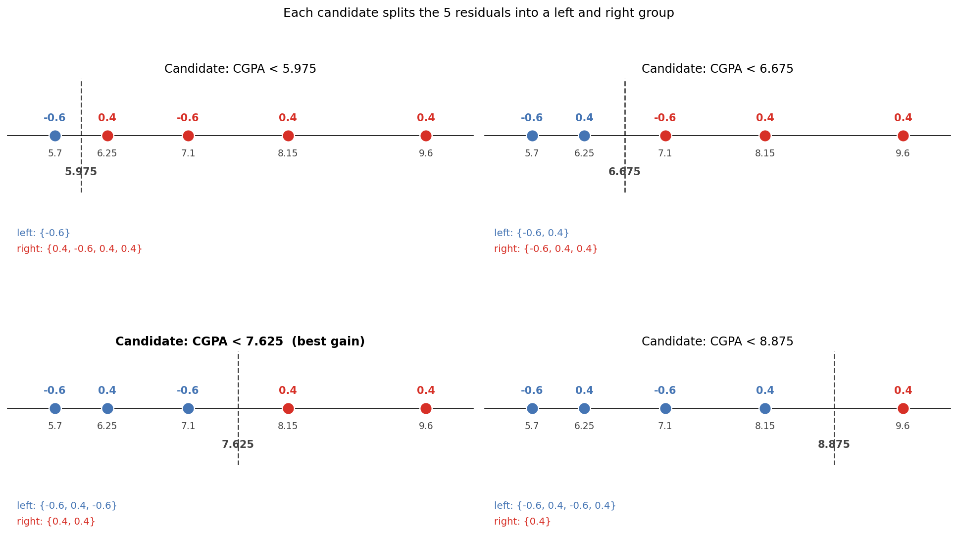
Every row's previous probability is 0.6, so every row contributes to a denominator. Working the first candidate in full, CGPA below 5.975:
- Left leaf,
{-0.6}: - Right leaf,
{0.4, -0.6, 0.4, 0.4}:
The left leaf scores high because it holds a single residual, and there's nothing for it to cancel against. That's the general pattern: residuals of the same sign in one leaf reinforce each other in the squared sum, residuals of opposite sign cancel out and drag the score down.
The same arithmetic for all four candidates:
| Split (CGPA below) | Left residuals | Right residuals | SSL | SSR | Gain |
|---|---|---|---|---|---|
| 5.975 | {-0.6} | {0.4, -0.6, 0.4, 0.4} | 1.500 | 0.375 | 1.875 |
| 6.675 | {-0.6, 0.4} | {-0.6, 0.4, 0.4} | 0.083 | 0.056 | 0.139 |
| 7.625 | {-0.6, 0.4, -0.6} | {0.4, 0.4} | 0.889 | 1.333 | 2.222 |
| 8.875 | {-0.6, 0.4, -0.6, 0.4} | {0.4} | 0.167 | 0.667 | 0.833 |
CGPA below 7.625 wins. Its right leaf is the only leaf in the table where every residual has the same sign and there's more than one of them, two s adding up to with nothing cancelling. The 6.675 split is the worst for the opposite reason: both of its leaves mix a with s, so both sums nearly cancel to .
The left child still holds three rows, and it could be split further by running the same search over its own candidates (5.975 and 6.675). This example stops at depth 1, a single split, to keep the arithmetic short and because boosting deliberately uses shallow trees. The first tree is:
CGPA < 7.625?
├── Yes → leaf: {5.70, 6.25, 7.10}   (residuals -0.6, 0.4, -0.6)
└── No  → leaf: {8.15, 9.60}         (residuals 0.4, 0.4)
6. Leaf Output Values
The leaf output formula is the similarity score without the square in the numerator, the same relationship as in regression:
With , this is exactly gradient boosting's leaf log-odds formula, which is why the output lands in log-odds space and can be added straight to the 0.405 baseline:
| Leaf | Residuals | Output |
|---|---|---|
| CGPA | {-0.6, 0.4, -0.6} | |
| CGPA | {0.4, 0.4} |
7. Stage 2: The Combined Prediction
The stage 2 model is the baseline plus the learning rate times the tree's output. XGBoost's default learning rate is :
- CGPA (5.70, 6.25, 7.10):
- CGPA (8.15, 9.60):
These are still log-odds, and a residual needs a probability, so each one goes through the sigmoid again: and . Subtracting from the actual label gives res2, and the table from Section 3 is now complete:
| CGPA | Placed? | pred1 (log-odds) | pred1 (prob) | res1 | pred2 (log-odds) | pred2 (prob) | res2 |
|---|---|---|---|---|---|---|---|
| 5.70 | 0 | 0.405 | 0.6 | -0.6 | 0.072 | 0.518 | -0.518 |
| 6.25 | 1 | 0.405 | 0.6 | 0.4 | 0.072 | 0.518 | 0.482 |
| 7.10 | 0 | 0.405 | 0.6 | -0.6 | 0.072 | 0.518 | -0.518 |
| 8.15 | 1 | 0.405 | 0.6 | 0.4 | 0.905 | 0.712 | 0.288 |
| 9.60 | 1 | 0.405 | 0.6 | 0.4 | 0.905 | 0.712 | 0.288 |
Comparing res1 against res2, four of the five residuals moved toward zero: twice, and twice. The exception is the CGPA 6.25 row, whose residual grew, . That's not an arithmetic slip; it falls straight out of the tree. The 6.25 student was placed, but a depth-1 tree can only split CGPA once, and the best single split lumps 6.25 in with its two unplaced neighbors (5.70 and 7.10). That leaf's residuals are mostly negative, so its output pushes all three rows toward "not placed," including the one row that should have gone the other way. A deeper tree (splitting that left leaf again) or later boosting stages are what eventually pull that row back.
8. Checking Against a Real XGBClassifier
There's no companion notebook for this example, so the hand arithmetic above is checked against a real XGBClassifier fit on the same five rows with matching settings: one tree, depth 1, , , the exact greedy split search, and a baseline probability of 0.6 (for binary classification base_score is given as a probability, and XGBoost converts it to log-odds 0.405 internally):
import numpy as np
from xgboost import XGBClassifier

cgpa = np.array([5.70, 6.25, 7.10, 8.15, 9.60]).reshape(-1, 1)
placed = np.array([0, 1, 0, 1, 1])

model = XGBClassifier(
    n_estimators=1, max_depth=1, learning_rate=0.3,
    reg_lambda=0, base_score=0.6,
    min_child_weight=0, gamma=0, tree_method="exact",
)
model.fit(cgpa, placed)
print(model.predict(cgpa, output_margin=True))  # log-odds
print(model.predict_proba(cgpa)[:, 1])          # probability
print(model.get_booster().get_dump(with_stats=True)[0])
[0.07213175 0.07213175 0.07213175 0.9054651 0.9054651 ]
[0.51802516 0.51802516 0.51802516 0.7120713 0.7120713 ]
0:[f0<7.625] yes=1,no=2,missing=1,gain=2.22222233,cover=1.19999993
1:leaf=-0.333333403,cover=0.719999969
2:leaf=0.5,cover=0.479999989
Everything matches: the split lands at 7.625 with gain 2.222, the log-odds and probabilities match the pred2 columns, and the leaf values are the hand-derived outputs with the learning rate already applied (, ).
The tree dump also shows a quirk worth knowing about. The cover of each node is exactly the denominator from Section 4: 1.2 at the root, 0.72 and 0.48 in the leaves. XGBoost's min_child_weight hyperparameter (default 1) is a minimum on this cover, not on the number of rows. In regression every row contributes 1 to the cover, so the default is harmless there. In classification each row here contributes only 0.24, so no leaf of this 5-row dataset can reach a cover of 1, and with the default left in place XGBoost refuses to split at all. Dropping min_child_weight=0 from the code above produces a single-leaf "tree" (0:leaf=-2.98023259e-08), a stump with no split whose output is effectively zero. On a real dataset with thousands of rows this rarely matters, but it's the reason the hand calculation needs min_child_weight=0 to be reproduced, and it's why confidently classified rows (small ) count for less than uncertain ones when XGBoost decides whether a leaf is big enough.
9. Stage 3 and Beyond
From here the loop repeats with nothing new. Take CGPA and res2, build a second similarity-score tree the same way, compute its leaf outputs using the new previous probabilities (0.518 and 0.712, so rows no longer contribute equally to the denominator), and add it to the running total:
Convert to probabilities, compute res3, fit tree 3 on that, and keep going until the residuals are at or very close to zero.
10. What to Take Away
- XGBoost for classification uses the same flow as gradient boosting for classification: a log-odds baseline, residuals computed on probabilities, trees fit to those residuals, outputs added in log-odds space and scaled by a learning rate.
- The only new ingredient is how each tree is built: splits are chosen by maximizing gain , the same as in XGBoost regression.
- The classification similarity score is : the regression formula with each row counting as instead of 1.
- A leaf's output is , which with is exactly gradient boosting's leaf log-odds formula.
- The first tree's root similarity is always zero, because a baseline probability equal to the label mean produces residuals that sum to zero.
- A single boosting stage doesn't have to shrink every residual: a shallow tree can push a row the wrong way when it shares a leaf with rows of the other class.
- XGBoost's
min_child_weightlimits the sum of in a leaf, not its row count, so tiny classification datasets need it lowered to split at all.