
Ch.62: XGBoost for Regression, Worked by Hand
Inspired by: YouTube
The previous post covered XGBoost's flexibility, speed, and performance engineering at a high level without touching the one piece that's genuinely new: how its trees actually get built. This post fixes that, working a complete regression example by hand on a tiny dataset, then checking every number against a real fitted model.
1. Same Recipe, One New Ingredient
XGBoost solves a regression problem with the exact same skeleton as plain gradient boosting: start with a baseline (the mean of the target), fit a tree to the current residuals, scale that tree's output by a learning rate and add it to the running prediction, then repeat. If someone asks "how does XGBoost do regression," the honest one-line answer is "the same way gradient boosting does."
The one real difference is how each tree gets built. A vanilla decision tree picks splits using gini impurity, entropy, or variance reduction. XGBoost's trees use a different criterion entirely, one built around a quantity called the similarity score, which has a regularization term baked directly into it. That's the actual new mechanic this post works through.
2. The Data and the Stage 0 Baseline
A tiny placement dataset: 4 students, CGPA as the only input feature, package (in LPA) as the target.
| CGPA | Package |
|---|---|
| 6.7 | 4.5 |
| 9.0 | 11.0 |
| 7.5 | 6.0 |
| 5.0 | 8.0 |
Same as gradient boosting, stage 0 is just the mean of the target, no feature involved:
Every student gets predicted 7.375 regardless of CGPA, and the pseudo-residual for each row is actual minus predicted:
| CGPA | Package | prediction | Residual |
|---|---|---|---|
| 6.7 | 4.5 | 7.375 | -2.875 |
| 9.0 | 11.0 | 7.375 | 3.625 |
| 7.5 | 6.0 | 7.375 | -1.375 |
| 5.0 | 8.0 | 7.375 | 0.625 |
Worth noticing before moving on: these four residuals sum to exactly zero. That's not a coincidence specific to this dataset, subtracting the mean from every value always produces residuals that sum to zero, it's a direct consequence of what a mean is. This fact becomes useful in the next section.
3. The Similarity Score
To decide where to split, XGBoost computes a similarity score for whatever group of residuals sits at a node:
is the number of residuals in that group, and is a regularization hyperparameter (set to throughout this post, its actual effect on overfitting is worth its own post once the math behind it is derived). Squaring the summed residuals means a group of residuals that mostly cancel out (some positive, some negative) scores low, while a group that's mostly one-directional scores high, similarity here means "how much these residuals agree in sign and size," not similarity in the everyday sense.
Applying this to all four residuals together, at the root, before any split:
The root's similarity score is exactly zero, a direct consequence of Section 2's observation that the residuals sum to zero. This will matter in a moment: it means the "gain" calculation below simplifies for this particular tree's root.
4. Finding the Best Root Split
Splitting works exactly like a vanilla decision tree's threshold search: sort the feature, take the midpoint between every consecutive pair of values, and try each one as a candidate split.
Each candidate carves the four residuals into a different left/right pair:
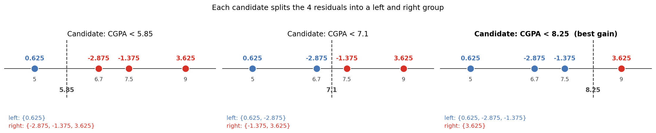
For each candidate, compute the similarity score of the left group (SSL) and right group (SSR), then the gain from splitting:
| Split (CGPA below) | Left residuals | Right residuals | SSL | SSR | Gain |
|---|---|---|---|---|---|
| 5.85 | {0.625} | {-2.875, 3.625, -1.375} | 0.391 | 0.130 | 0.521 |
| 7.1 | {-2.875, 0.625} | {3.625, -1.375} | 2.531 | 2.531 | 5.063 |
| 8.25 | {-2.875, -1.375, 0.625} | {3.625} | 4.380 | 13.141 | 17.521 |
Since (Section 3), gain here is just SSL + SSR, nothing to subtract. The split at CGPA below 8.25 wins by a wide margin, mostly because it isolates the single largest residual (3.625, the CGPA = 9.0 row) into its own leaf, and an unshared residual squared over produces a large similarity score.
5. Growing a Second Level
The right side of that split (CGPA 8.25, just the one row with residual 3.625) has nothing left to split. The left side has three rows and two remaining candidate thresholds, 5.85 and 7.1:
| Split (CGPA below) | Left residuals | Right residuals | SSL | SSR | Gain |
|---|---|---|---|---|---|
| 5.85 | {0.625} | {-2.875, -1.375} | 0.391 | 9.031 | 5.042 |
| 7.1 | {-2.875, 0.625} | {-1.375} | 2.531 | 1.891 | 0.042 |
5.85 wins clearly, again because it isolates a lone residual (0.625, the CGPA = 5.0 row) into its own single-row leaf. The finished tree, capped at depth 2 (XGBoost's own default is depth 6, but a 4-row toy dataset has no business growing that deep):
CGPA < 8.25?
├── No  → leaf: {9.0}                    (residual 3.625)
└── Yes → CGPA < 5.85?
          ├── Yes → leaf: {5.0}           (residual 0.625)
          └── No  → leaf: {6.7, 7.5}      (residuals -2.875, -1.375)
6. Leaf Output Values
Once the structure is fixed, each leaf needs an actual number to output. The formula is close to the similarity score's numerator, but without the square:
With , this is just the average of the residuals in that leaf, same as a vanilla regression tree:
| Leaf | Residuals | Output |
|---|---|---|
| CGPA 8.25 | {3.625} | 3.625 |
{-2.875, -1.375} | -2.125 | |
| CGPA | {0.625} | 0.625 |
7. Assembling the Stage 1 Combined Model
The running prediction updates the same way it does in plain gradient boosting, baseline plus learning rate times the tree's output for that row. XGBoost's default learning rate () is :
| CGPA | Package (actual) | (baseline pred.) | Old residual (Section 2) | Leaf output | New residual | |
|---|---|---|---|---|---|---|
| 6.7 | 4.5 | 7.375 | -2.875 | -2.125 | -2.2375 | |
| 9.0 | 11.0 | 7.375 | 3.625 | 3.625 | 2.5375 | |
| 7.5 | 6.0 | 7.375 | -1.375 | -2.125 | -0.7375 | |
| 5.0 | 8.0 | 7.375 | 0.625 | 0.625 | 0.4375 |
Compare the new residuals against Section 2's originals, every single one shrank toward zero (-2.875 → -2.2375, 3.625 → 2.5375, -1.375 → -0.7375, 0.625 → 0.4375). That's the whole point of a boosting stage: nudge every prediction a bit closer to correct, then repeat with a second tree fit on these smaller residuals, and a third, and so on.
Hand arithmetic across four sections is exactly the kind of thing worth double-checking against real code rather than trusting by eye. Replicating the exact-greedy split search above in plain Python and comparing it to a real XGBRegressor fit with matching hyperparameters:
from xgboost import XGBRegressor
import numpy as np

cgpa = np.array([6.7, 9.0, 7.5, 5.0]).reshape(-1, 1)
package = np.array([4.5, 11.0, 6.0, 8.0])

model = XGBRegressor(
    n_estimators=1, max_depth=2, learning_rate=0.3,
    reg_lambda=0, base_score=package.mean(),
    min_child_weight=0, gamma=0, tree_method="exact",
)
model.fit(cgpa, package)
print(model.predict(cgpa))
[6.7375 8.4625 6.7375 7.5625]
That matches the table's hand-derived predictions exactly, confirming the similarity-score/gain/leaf-output formulas above are the actual mechanism, not just an approximation of one.
8. A Note on How Splits Get Searched
The threshold search in Section 4 and Section 5, sort the feature, try the midpoint of every consecutive pair, is called the exact greedy algorithm, and it's what XGBoost's original paper describes as the default approach: accurate, since it genuinely checks every possible split, but expensive on a feature with millions of distinct values, since every one of those becomes a candidate. For large datasets, XGBoost falls back to an approximate algorithm instead, which buckets candidate splits rather than trying every single value, similar in spirit to the quantile-based binning covered in the flexibility/speed overview. That approximate method deserves its own dedicated treatment rather than a mention here.
9. Multiple Features and Categorical Splits
The toy dataset above has exactly one feature. A real placement dataset would have several, CGPA alongside 12th-grade marks, internship count, and so on, and it's worth working out how the split search changes once there's more than one column, and once a column isn't numeric.
More than one numeric feature. The search doesn't change in kind, only in scope. This is the same extension covered for vanilla regression trees: the exact-greedy sweep from Section 4, sort the feature, test every midpoint, runs independently on every numeric column. Each feature comes back with its own best candidate threshold and the gain that threshold achieves. Whichever feature's best gain is highest wins the node, and its threshold becomes the split condition. A tree built on CGPA and 12th-grade marks might split on CGPA at the root and 12th-grade marks two levels down, or never touch 12th-grade marks at all if CGPA keeps winning the gain comparison at every node it's tried against.
A binary categorical feature. With only two categories (say, an internship column coded 0/1), there's exactly one possible way to divide the rows, left gets one category, right gets the other. No sweep is needed: compute the gain for that single split and treat it exactly like any other feature's best candidate in the comparison above.
A multi-class categorical feature. With categories and no natural ordering to sort by, the midpoint-sweep search doesn't directly apply, there's no "midpoint" between, say, a Computer Science and a Mechanical degree branch. Trying every possible way to divide unordered categories into two groups is exponential ( candidate splits), too expensive to brute-force once grows past a handful. The way around it, used by XGBoost's native categorical support and by LightGBM: sort the categories by their mean target value (or mean residual, in a boosting context) within that node, then run the exact same midpoint sweep from Section 4 over that sorted order, as if the categories were now a numeric feature. This is provably optimal for a single split, a result that goes back to Fisher's work on partitioning categorical predictors, and it turns an exponential search into a linear one. The more common approach in practice, and the only one older XGBoost versions support without enable_categorical=True, is simpler still: one-hot encode the column into binary features upfront and let each one compete in the ordinary numeric split search above.
10. What to Take Away
- XGBoost's regression procedure is structurally identical to plain gradient boosting: baseline (mean), fit a tree to the residuals, scale by a learning rate, update, repeat.
- The actual difference is how each tree is built: splits are chosen by maximizing gain (SSL + SSR - SS_parent), where similarity score is , not by gini, entropy, or variance reduction.
- A leaf's output value is , the same as a plain average when .
- Residuals from a mean baseline always sum to zero, which is why a stage-1 tree's root similarity score is always zero, and gain reduces to just SSL + SSR for that first tree.
- The default learning rate is and the default max tree depth is , though a small toy dataset has no reason to use either default at full strength.
- This exact-greedy split search (try every possible threshold) is one of two split-finding strategies XGBoost supports, the other, an approximate quantile-based method for large datasets, is a topic on its own.
- With multiple features, every feature runs its own gain-maximizing search independently and the best gain across all of them wins the node; categorical features join that same search either by one-hot encoding or by sorting categories on mean target value first.