Ch.54: AdaBoost, Geometric Intuition

By Ayush Arora•2026-09-25•8 min read

Inspired by: YouTube

Bagging and random forest train every base model independently and let them vote as equals. Boosting is the other big branch of ensemble learning: models are trained one after another, each one specifically told which points the previous one got wrong, and the final prediction weighs each model's opinion by how good it actually was. AdaBoost (Adaptive Boosting) is the first and oldest boosting algorithm, and everything later boosting methods (gradient boosting, XGBoost) build on shows up here first in its simplest form.

This is a 4-part series, and this post covers only the first video: the geometric intuition, no weight-update formula yet. The exact math for computing alpha and for up-sampling gets its own follow-up post once that video is transcribed; for now the goal is to be able to look at the diagram below and know why AdaBoost draws the boundary it draws.

1. Two Building Blocks First

Weak learner. A weak learner is a model whose accuracy is only just above random guessing, about 50% for a binary problem, the same as calling a coin flip. That sounds useless on its own, but boosting's whole premise is that combining many weak learners, each one nudged to focus on the previous one's mistakes, produces one strong learner with accuracy in the 90s. A single weak learner is nearly worthless; a sequence of them, weighted by how well each one did, is not.

Decision stump. AdaBoost can technically use any weak learner, but in practice it almost always uses decision stumps: a decision tree with max_depth=1, meaning exactly one split. A stump can only ever draw one line parallel to one axis, either the CGPA axis or the IQ axis in the running example, never a diagonal or a combination, so on its own it's a bad classifier by construction, which is exactly the "weak learner" property AdaBoost wants. Between the two possible axis-aligned splits, the stump picks whichever one reduces entropy the most, same rule as any decision tree split.

from sklearn.tree import DecisionTreeClassifier
import pandas as pd
 
df = pd.DataFrame()
df['X1'] = [1, 2, 3, 4, 5, 6, 6, 7, 9, 9]
df['X2'] = [5, 3, 6, 8, 1, 9, 5, 8, 9, 2]
df['label'] = [1, 1, 0, 1, 0, 1, 0, 1, 0, 0]
 
dt1 = DecisionTreeClassifier(max_depth=1)
dt1.fit(df[['X1', 'X2']], df['label'])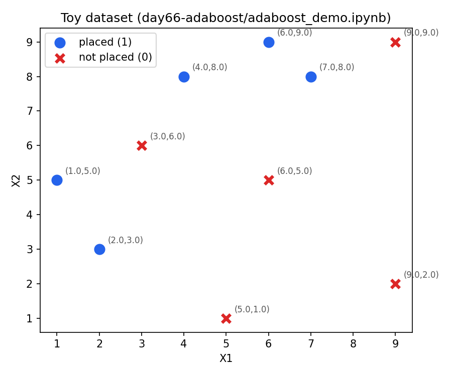

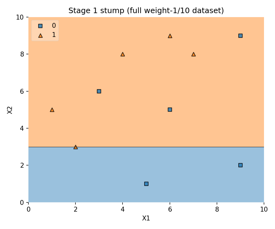
Scatter plot of 10 points on X1/X2 axes, 6 blue circles labeled placed (1) and 4 red X markers labeled not placed (0), scattered without a clean linear separation

Decision region plot for a single decision stump, one horizontal split, orange region above the line, blue region below, with several misclassified points visible on the wrong side of the split

One split, a handful of points end up on the wrong side. That's a decision stump: cheap to fit, easy to interpret (a single split tells you plainly which feature and threshold it used), and deliberately weak.

2. Why Labels Are +1/-1, Not 0/1

Most binary classifiers use 0 and 1 for the two classes. AdaBoost's math instead uses +1 and -1, positive points get +1, negative points get -1. Why that specific choice isn't explained yet, it clicks once you see the final combination rule in Section 4, a weighted sum of +1/-1 votes whose sign gives the class directly. For now, just note the convention: this is one of three things worth knowing before the algorithm itself starts (the other two are weak learners and decision stumps above).

3. Stage-Wise Additive Modeling

You'll often see AdaBoost described as a stage-wise additive model, which is just two words for the training loop:

Additive: the final model is a weighted sum of several weak learners, not one model replacing another.
Stage-wise: those weak learners are added one at a time, in stages, each new one built on top of what the previous stages got wrong, never revisited or retrained afterward.

4. The Geometric Walkthrough

Take a small dataset: a handful of students, their CGPA, their IQ, and whether they got placed. Every row starts with equal weight, nobody gets extra attention yet.

Stage 1. Fit one decision stump on the full, equally-weighted dataset. Whichever stump reduces entropy the most gets picked, it makes some mistakes (it's only one line, it has to), and the model itself is told: your job here is done, now here's your own weight in the final vote, based on how well you did.

Up-sample the mistakes. Instead of retraining on the same data, the points the first stump got wrong are given more weight, more importance, so the next stump's training data is skewed toward exactly what the previous one missed. How that reweighting is computed isn't covered yet, that's next post's job, the geometric idea is just: wrong points get bigger.

Stage 2, stage 3, ... A new stump is fit on this up-weighted data. It usually draws a different split, since the data it's seeing has changed emphasis, correctly handling some of stage 1's mistakes while making a few new ones of its own. It gets its own weight based on its own performance, and the process repeats: up-sample this stage's mistakes, fit the next stump.

Here's the whole loop, matching the board sketch from the video:

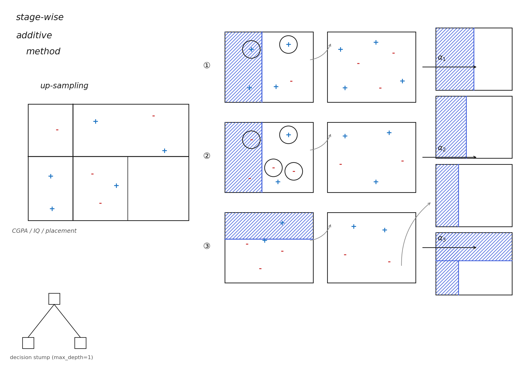
Diagram of the AdaBoost stage-wise additive method. A decision stump icon (root node splitting into two leaves) labeled max_depth=1. Below it, an up-sampling panel showing a small dataset split into quadrants with plus and minus points. Three numbered stage rows: each row shows a left panel (data with a stump's split line, one region hatched, misclassified points circled), an arrow into a right panel (the same points up-sampled for the next stage), and an alpha arrow (alpha-1, alpha-2, alpha-3) pointing to a column of four boxes on the right that show the combined decision region getting progressively refined as more stumps are added, ending in a boundary with a stepped, non-rectangular shape

Each row is one stage: a stump splits the current (reweighted) data, its mistakes get circled and up-sampled into the next row's data, and its alpha feeds into the combined boundary on the right, which sharpens with every stage added.

5. Combining the Stumps Into One Prediction

With, say, three stumps trained this way, the final AdaBoost prediction is:

H(x) = \text{sign}\left(\alpha_1 h_1(x) + \alpha_2 h_2(x) + \alpha_3 h_3(x)\right)

Each $h_i(x)$ is that stump's vote as +1 or -1, multiplied by that stump's own alpha (a well-performing stump gets a bigger alpha and a louder vote), summed across all stumps, and the sign of the total is the final class. This is exactly why +1/-1 labels matter, from Section 2: a correct +1 vote and a correct -1 vote both push the sum in the right direction, so summing weighted votes and taking the sign works cleanly.

A worked example, straight from the video. For a new student with CGPA 7.5 and IQ 81: stump 1 (weight $\alpha_1 = 2$ ) predicts -1, stump 2 (weight $\alpha_2 = 10$ ) predicts +1, stump 3 (weight $\alpha_3 = 1$ ) predicts -1.

2(-1) + 10(1) + 1(-1) = -2 + 10 - 1 = 7

7 is positive, sign(7) = +1, so the model predicts placement. Note that stump 2 alone was wrong about the magnitude mattering, it carries $\alpha_2 = 10$ , ten times stump 1's weight, because it's the most trustworthy of the three; its single +1 vote outweighs the other two -1 votes combined.

The geometric picture. Stack all three stumps' decision regions on top of each other and the overlap produces a boundary none of them could draw alone, closer to where the actual placed/not-placed split in the data really is. Add more stumps and that boundary keeps refining. That's the entire geometric intuition: several weak, single-line classifiers, each correcting for what the last one missed, combine into one strong, more flexible boundary.

6. What to Take Away

A weak learner is only just better than a coin flip; AdaBoost's default weak learner is a decision stump, a depth-1 tree that can only draw one axis-aligned split.
Boosting is stage-wise (models are added one at a time) and additive (the final prediction is their weighted sum), the opposite of bagging's equal-vote "democracy."
Each stage does two things: gets its own alpha based on how well it performed, and up-samples its own mistakes so the next stage's stump focuses on them.
The final prediction is sign(alpha1*h1 + alpha2*h2 + alpha3*h3 + ...), which is exactly why votes are +1/-1 rather than 1/0.
Stacking several single-line splits geometrically produces a boundary none of them could draw individually.

Next: the actual math behind AdaBoost's weight update, exactly how alpha is calculated and how the up-sampling works, once that video is transcribed.

View all chapters in Machine Learning Algorithms →