Ch.64: Deriving XGBoost's Formulas From Scratch

Inspired by: YouTube

The regression and classification walkthroughs used two formulas without justifying either: the similarity score, $(\sum \text{residuals})^2 / (n + \lambda)$ for regression and $(\sum \text{residuals})^2 / (\sum p(1-p) + \lambda)$ for classification, and the matching leaf output formula, the same numerator without the square. Both were presented as "this is what you compute," with a promise to come back to where they came from. This post is that derivation, starting from XGBoost's actual objective function and ending at the exact formulas used in both earlier posts.

1. The Objective Function, Built Up Stage by Stage

Gradient boosting's additive structure means a model after $t$ stages is a sum of functions, $\hat y_i = \sum_{k=1}^{t} f_k(x_i)$, where each $f_k$ is one fitted tree (or, for $f_1$, a constant baseline). Every one of those trees makes some amount of error, and the quantity you want to minimize at any stage combines that error with a penalty on model complexity:

The regularization term $\Omega(f)$ only applies to decision trees, not to a constant baseline, since a flat number has no leaves to penalize. For the single-tree case this is:

$T$ is the number of leaves in that tree, $w_j$ is leaf $j$'s output value (its "weight"), and $\gamma$, $\lambda$ are two separate regularization knobs: $\gamma$ penalizes having too many leaves, $\lambda$ penalizes leaves with large output magnitudes. This is the piece the XGBoost overview referred to as "a regularization term baked directly into the loss."

At stage $t$, every tree before the current one is already fixed, so $\hat y_i^{(t)} = \hat y_i^{(t-1)} + f_t(x_i)$ splits the objective into "everything already accounted for" and "the one new tree":

The goal at every stage is the same: find the $f_t$ (equivalently, the leaf weights of the $t$-th tree) that minimizes this expression. That makes it an optimization problem, the same flavor as fitting $m$ and $b$ in linear regression by minimizing mean squared error, just with a far less convenient function to minimize.

2. Why This Can't Be Differentiated Directly

Ordinary optimization differentiates the objective with respect to the parameter being solved for, sets that derivative to zero, and solves. In linear regression, the loss as a function of $m$ and $b$ traces out a smooth parabola, differentiable everywhere, which is exactly what makes that route work.

$f_t(x_i)$ here is a decision tree, and a decision tree's output is piecewise constant: the same output for every row that lands in a given leaf, then a sudden jump for rows in the next leaf over. Fitting the same two curves, a line and a shallow tree, to one dataset makes the shape difference concrete:

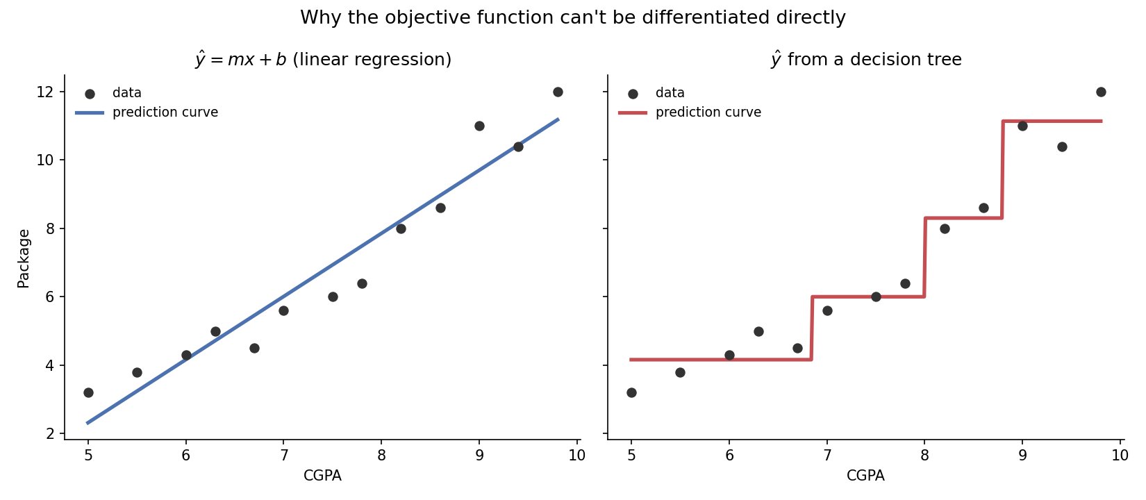
A straight line is differentiable at every point. The staircase is not, at each jump the slope is undefined, there's no single tangent line to speak of. Since $\hat y_i^{(t)}$ is built out of $f_t(x_i)$, plotting the objective function against $f_t(x_i)$ inherits that same jaggedness instead of a clean parabola. Partial differentiation with respect to $f_t(x_i)$ breaks down at exactly the points where it would be needed.

3. Taylor Series: Smoothing a Function Into a Polynomial

The fix is to approximate the non-differentiable objective with something that is differentiable, close enough to be useful, close enough to be trustworthy. The Taylor series is the standard tool for exactly this: given a complicated function $f(x)$ and a nearby point $a$, it builds a polynomial approximation out of $f$'s derivatives at $a$:

Each additional term tightens the approximation around $a$. Expanding $e^x$ around $a=0$ term by term:

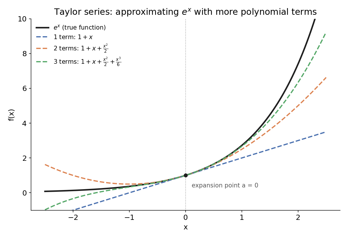
With one term the fit only holds very close to $a=0$; with three terms it tracks the true curve over a visibly wider range. That's the general trade: more terms buys more accuracy, farther from $a$. XGBoost's objective function stops at two terms, a second-order (quadratic) approximation, which turns out to be exactly enough.

4. Applying the Taylor Expansion to the Objective

Treat $l(y_i, \hat y_i^{(t-1)} + f_t(x_i))$ as the function being approximated, with $x = \hat y_i^{(t-1)} + f_t(x_i)$ and the expansion point $a = \hat y_i^{(t-1)}$, the prediction already locked in before this tree gets added. $x - a$ is then just $f_t(x_i)$, so the second-order expansion is:

where $g_i$ and $h_i$ are the first and second derivatives of the loss with respect to the previous prediction, evaluated at $\hat y_i^{(t-1)}$:

$g_i$ is called the gradient, $h_i$ the Hessian (the standard name for a second derivative in optimization). Substituting this approximation into the objective:

The next move is to notice that $l(y_i, \hat y_i^{(t-1)})$ doesn't involve $f_t(x_i)$ at all, it's a fixed number by the time this tree is being fit. Since the entire point is to differentiate with respect to $f_t(x_i)$ and that term vanishes under differentiation anyway, it can be dropped without changing the answer:

Checking this against the paper confirms it line for line: a gradient term, a Hessian term, and the regularization term, nothing else.

5. From Rows to Leaves

$\Omega(f_t)$ is still sitting unexpanded. Writing it out:

There are now two different summations, one over rows ($i = 1$ to $n$), one over leaves ($j = 1$ to $T$), and they need to become one. The bridge is that $f_t(x_i)$, the tree's output for row $i$, is just the output of whichever leaf row $i$ lands in. If $I_j$ denotes the set of row indices that fall into leaf $j$, then summing over all rows one at a time is equivalent to grouping rows by leaf first and summing within each group:

Reusing the regression walkthrough's finished tree makes this concrete. That tree has three leaves: $I_1 = \{\text{CGPA} \geq 8.25\}$ (row with CGPA 9.0), $I_2 = \{5.85 \leq \text{CGPA} < 8.25\}$ (rows with CGPA 6.7 and 7.5), $I_3 = \{\text{CGPA} < 5.85\}$ (row with CGPA 5.0). Summing $g_i f_t(x_i)$ over all four rows directly, or summing it leaf by leaf and then adding the three leaf totals together, reach the identical number, the rows are just visited in a different order.

Within a single leaf $j$, every row shares the same tree output, $f_t(x_i) = w_j$ for every $i \in I_j$, by definition of what a leaf is. That lets $w_j$ be pulled out of the inner sum entirely:

This used the fact that the $\lambda \sum w_j^2 / 2$ term already sums over $j$, so its $j$-th piece, $\frac{1}{2}\lambda w_j^2$, folds directly into the $j$-th leaf's bracket. Writing $G_j = \sum_{i \in I_j} g_i$ and $H_j = \sum_{i \in I_j} h_i$ for brevity:

Every term here is a function of a single leaf's weight $w_j$, nothing couples one leaf's weight to another's. That's what makes the next step possible.

6. Solving for the Optimal Leaf Weight

Each leaf's contribution, $G_j w_j + \frac{1}{2}(H_j + \lambda) w_j^2$, is a plain quadratic in $w_j$, exactly the shape a parabola takes, so it can be minimized the ordinary way: differentiate with respect to $w_j$, set to zero, solve.

This is the general leaf weight formula, valid for any differentiable loss function, with the specific loss only entering through $G_j$ and $H_j$. To check it reproduces the regression and classification formulas used earlier, it just needs $g_i$ and $h_i$ for each loss:

Regression, squared error $l(y, \hat y) = \frac{1}{2}(y-\hat y)^2$:

Classification, log loss with $\hat y$ in log-odds space and $p_i = \text{sigmoid}(\hat y_i^{(t-1)})$ (the same conversion used in gradient boosting for classification):

Both of these are checkable with symbolic differentiation rather than by hand:

import sympy as sp
 
y, yhat, z = sp.symbols('y yhat z')
 
# regression: L = 1/2 (y - yhat)^2
L_reg = sp.Rational(1, 2) * (y - yhat)**2
print("g_reg:", sp.diff(L_reg, yhat))        # yhat - y
print("h_reg:", sp.diff(L_reg, yhat, 2))     # 1
 
# classification: L = log loss, z is log-odds, p = sigmoid(z)
p = 1 / (1 + sp.exp(-z))
L_cls = -(y * sp.log(p) + (1 - y) * sp.log(1 - p))
g_cls = sp.simplify(sp.diff(L_cls, z))
h_cls = sp.simplify(sp.diff(L_cls, z, 2))
print("g_cls:", g_cls)
print("h_cls:", h_cls)

g_reg: -y + yhat
h_reg: 1
g_cls: (-y + (1 - y)*exp(z))/(exp(z) + 1)
h_cls: exp(z)/(exp(2*z) + 2*exp(z) + 1)

h_cls simplifies to $p(1-p)$ (since $e^z/(1+e^z)^2 = p(1-p)$ once $p = e^z/(1+e^z)$), and g_cls simplifies to $p - y$ by the same substitution, confirming both by hand matches what sympy returns.

Plugging these into $w_j^* = -G_j/(H_j+\lambda)$:

Both are exactly the leaf output formulas used without proof in the regression and classification posts. The "sum of residuals" in both earlier posts was always $-G_j$, and the "$n$" or "$\sum p(1-p)$" in the denominator was always $H_j$.

7. The Minimum Loss, and Where the Similarity Score Comes From

$w_j^*$ is the weight that minimizes each leaf's contribution to the objective, but it doesn't yet say what that minimum value is. Substituting $w_j^*$ back into $G_j w_j + \frac{1}{2}(H_j+\lambda)w_j^2$:

Summed across all $T$ leaves, the minimum achievable objective for a given tree structure is:

The paper calls this a structure score, a single number that says how good a candidate tree shape is, lower is better since it's a loss. Flip the sign and drop the constant $-\frac{1}{2}$ and $\gamma T$ (neither affects which of several candidate splits scores highest, since a positive constant multiplier and an additive term that's identical across candidates can't change which one wins), and what's left is:

For a single leaf (T=1), this is $(\sum g_i)^2 / (\sum h_i + \lambda)$. Substituting $g_i = -\text{residual}_i$ for regression gives $(\sum \text{residual}_i)^2/(n+\lambda)$, exactly the regression similarity score. Substituting the classification $g_i, h_i$ gives $(\sum \text{residual}_i)^2/(\sum p(1-p)+\lambda)$, exactly the classification version. Both formulas trace back to the same two-line substitution, the only thing that ever changes between regression and classification is what loss function $g_i$ and $h_i$ come from.

8. From Similarity Score to Split Gain

A split takes one leaf (the parent) and replaces it with two (left and right child). Using $\mathcal{L}^*$ from Section 7, the loss before splitting (one leaf, $T=1$) is:

and the loss after splitting (two leaves, $T=2$) is:

A split is worth making exactly when it reduces the loss, so the quantity that matters is $\mathcal{L}^*_{\text{parent}} - \mathcal{L}^*_{\text{children}}$:

This is exactly the split criterion the regression and classification posts used, $\text{SSL} + \text{SSR} - \text{Similarity}_{\text{parent}}$, with two differences made explicit here: an overall factor of $\frac{1}{2}$, which doesn't change which candidate split wins since every candidate gets scaled the same way, and a $-\gamma$ term, set to zero in both earlier posts' worked examples. That $-\gamma$ is not cosmetic in general: it's the same $\gamma$ hyperparameter that sets a minimum required gain before a split is allowed to happen at all. A candidate split whose raw $\frac{1}{2}[\text{SSL}+\text{SSR}-\text{SS}_P]$ doesn't clear $\gamma$ gets rejected outright, regardless of how it compares to other candidates, which is the exact mechanism behind XGBoost's pruning behavior.

9. What to Take Away

• XGBoost's objective at stage $t$ is loss on the current prediction plus a regularization term on the newest tree, $\gamma T + \frac12 \lambda \sum w_j^2$, that penalizes both leaf count and leaf weight magnitude.
• That objective is non-differentiable in closed form with respect to the new tree, because a tree's output is piecewise constant, so a second-order Taylor expansion (around the previous stage's prediction) replaces it with a differentiable quadratic approximation.
• The expansion introduces $g_i$ (gradient, first derivative of the loss) and $h_i$ (Hessian, second derivative), the only place the specific loss function enters the rest of the derivation.
• Regrouping the per-row sum into a per-leaf sum, using $f_t(x_i) = w_j$ for every row in leaf $j$, turns the objective into an independent quadratic for each leaf's weight.
• Minimizing each leaf's quadratic gives $w_j^* = -G_j/(H_j+\lambda)$, which reduces to $\sum\text{residual}/(n+\lambda)$ for squared error and $\sum\text{residual}/(\sum p(1-p)+\lambda)$ for log loss, exactly the leaf output formulas used without derivation in the regression and classification posts.
• Plugging $w_j^*$ back into the objective gives a structure score for the whole tree; comparing a parent leaf's score against its two children's scores (after a split) produces the gain formula, $\frac12[\text{SSL}+\text{SSR}-\text{SS}_P] - \gamma$, the earlier posts' simplified $\text{SSL}+\text{SSR}-\text{SS}_P$ with the constant factor and the $\gamma$ pruning threshold made explicit.