Ch.39: Decision Tree Hyperparameters

Inspired by: YouTube

An unconstrained decision tree will keep splitting until every leaf is pure, or has just one row left. That gives it a well-earned reputation as a high-variance algorithm: left alone, it memorizes the training set, entropy at the root but zero at every leaf, and then fails to generalize to anything it hasn't seen. sklearn's DecisionTreeClassifier exposes a handful of hyperparameters that exist for exactly one reason: to stop the tree from growing that far.

1. Overfitting and Underfitting, the Two Failure Modes

A tree that's grown too deep has overfit: near-perfect training accuracy, visibly worse test accuracy, and a decision boundary with tiny islands carved out for single stray points. A tree that's cut off too early has underfit: it hasn't captured the real shape of the data and performs poorly on both training and test sets. Every hyperparameter below is a knob between these two failure modes, and tuning them is the practical answer to the question ch37 left open: when should splitting stop?

The demo dataset throughout is sklearn's make_moons, two interleaved, non-linearly-separable classes with some added noise, split 70/30 into train and test:

from sklearn.datasets import make_moons
from sklearn.model_selection import train_test_split
 
X, y = make_moons(n_samples=300, noise=0.25, random_state=42)
X_train, X_test, y_train, y_test = train_test_split(
    X, y, test_size=0.3, random_state=42
)

2. max_depth

The most direct lever: how many questions deep the tree is allowed to go from root to leaf. Left at its default (None), the tree grows until every leaf is pure, no matter how deep that requires.

from sklearn.tree import DecisionTreeClassifier
 
for depth in [1, 4, None]:
    clf = DecisionTreeClassifier(max_depth=depth, random_state=42)
    clf.fit(X_train, y_train)
    print(depth, clf.score(X_train, y_train), clf.score(X_test, y_test))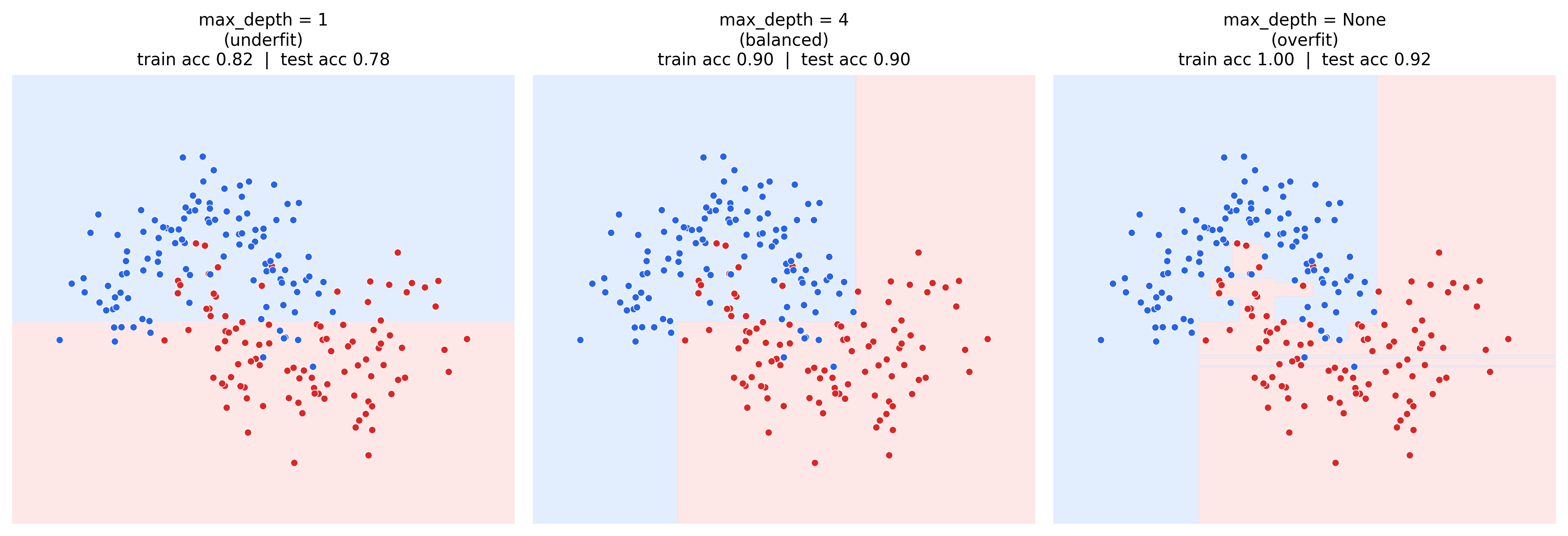

max_depth = 1 is a single axis-aligned cut, it can't do much better than guess which half of the plane each moon mostly falls in. max_depth = None chases every noisy point, including ones that shouldn't be trusted, carving out small islands that hurt more than they help on new data. max_depth = 4 sits in between: close to the actual moon-shaped boundary, and (in this run) matched train/test accuracy rather than a gap between them. Small max_depth underfits, large or unset max_depth overfits, and the right value is a balance found by comparing train and test scores, not read off a formula.

3. criterion: Gini vs. Entropy

The split-quality measure introduced in ch38, Gini impurity by default, entropy as the alternative. Sweeping max_depth against test accuracy with each:

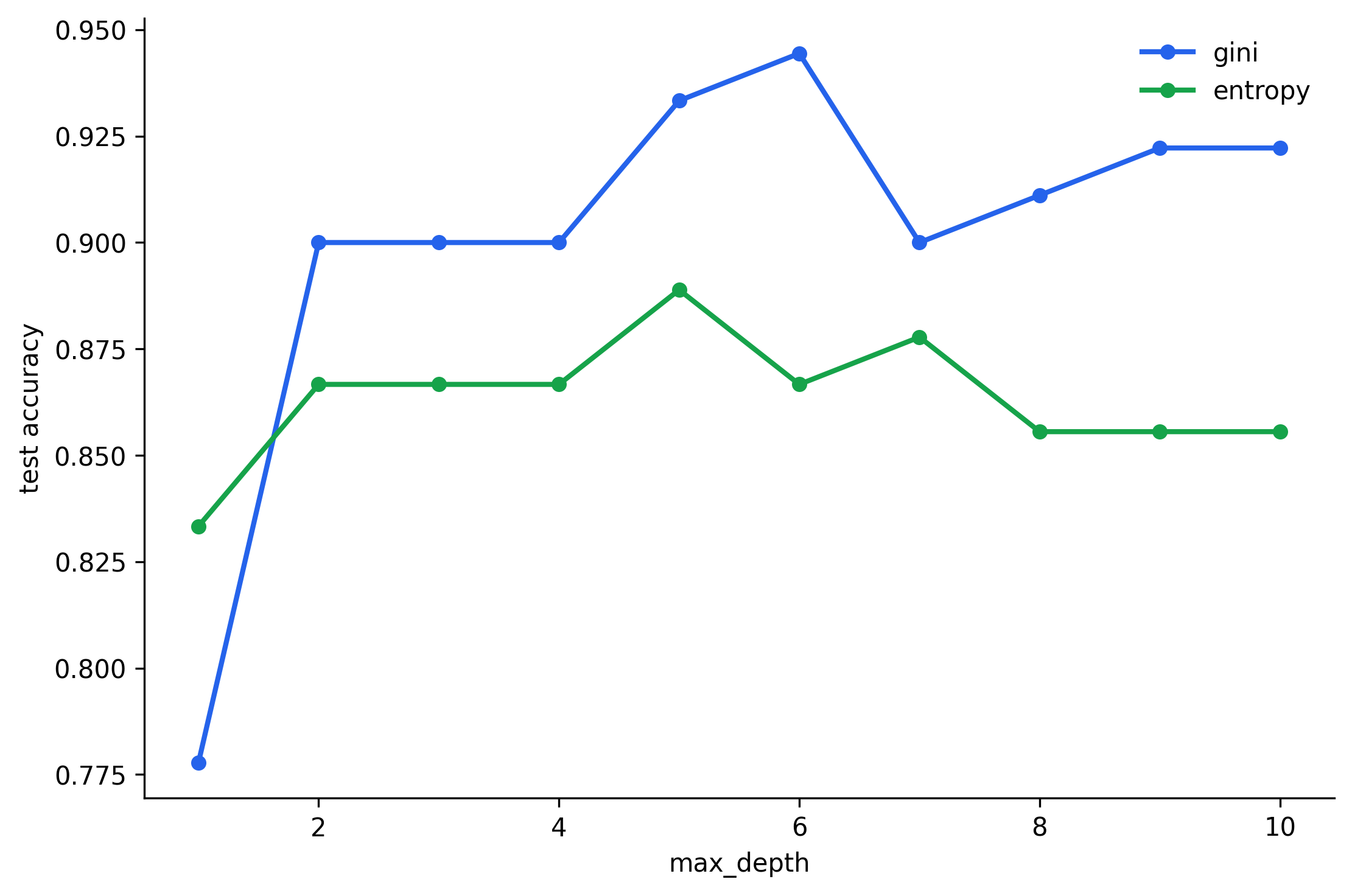
The two curves track each other closely, gini criterion peaked at 0.944 test accuracy (depth 6) versus entropy's peak of 0.889 (depth 5) in this run, but the shapes of both curves are nearly identical. In practice the choice rarely moves accuracy by much; gini is the default because it's cheaper to compute (no logarithm), and that's the only real reason to prefer it.

4. splitter: Best vs. Random

By default (splitter="best"), a node checks every feature and every candidate threshold on that feature, and picks whichever split gives the highest information gain. splitter="random" instead picks one random feature at each node and searches for the best threshold only on that one, trading a slightly worse-fitting tree for less overfitting, since the randomness stops the tree from over-committing to whichever feature looks marginally best on this particular training sample. It's a lighter-weight regularizer than the size-based hyperparameters below, useful mainly as a quick thing to try, not something with a generally "correct" setting.

5. min_samples_split and min_samples_leaf

Both hyperparameters stop a split from happening once a node's row count gets too small, but they check the count on different sides of the split:

• min_samples_split (default 2): a node needs at least this many rows before it's allowed to split at all.
• min_samples_leaf (default 1): after a split, both resulting children must end up with at least this many rows, or the split doesn't happen.

min_samples_leaf is the more common one to tune, since it directly bounds how small (and how easily swayed by one or two noisy points) any single leaf can be:

for leaf in [1, 5, 20]:
    clf = DecisionTreeClassifier(min_samples_leaf=leaf, random_state=42)
    clf.fit(X_train, y_train)
    print(leaf, clf.score(X_train, y_train), clf.score(X_test, y_test))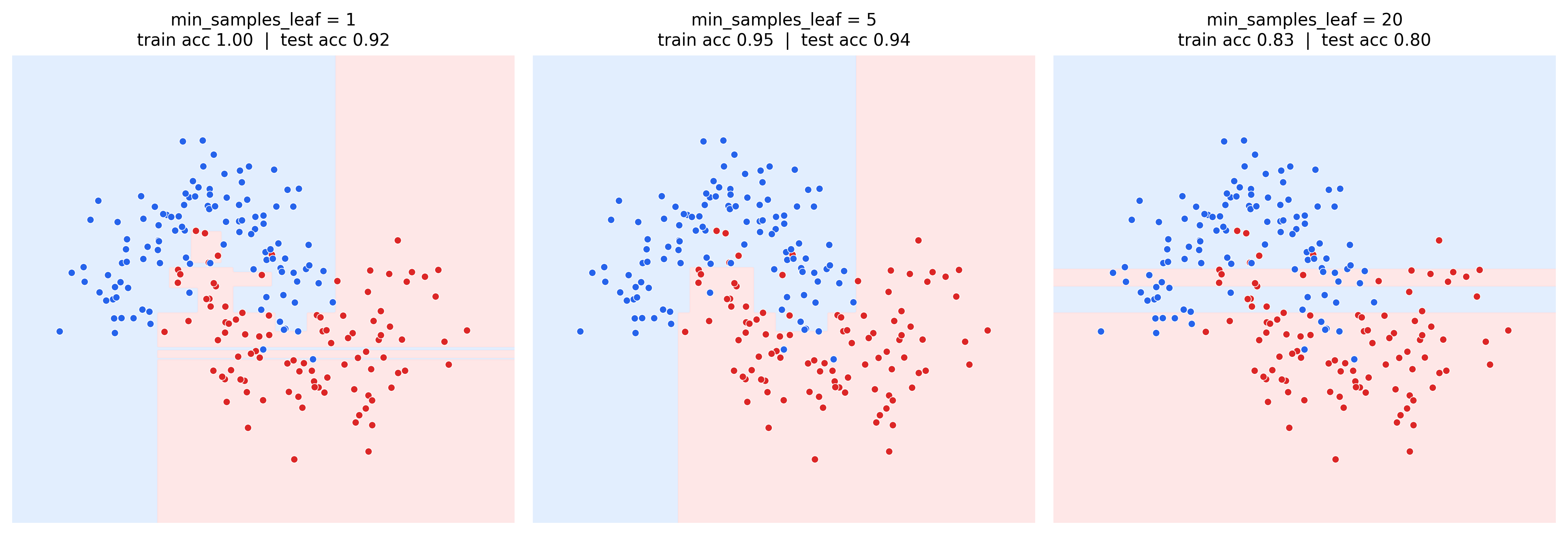

min_samples_leaf = 1 lets a leaf form around a single point, the small-islands overfitting pattern again (train 1.00, test 0.92). Raising it to 5 smooths those islands away while keeping the two-moon shape largely intact (train 0.95, test 0.94). Pushed to 20 the tree can no longer represent the moon curve at all and coarsens into wide horizontal bands, underfitting both sets (train 0.83, test 0.80). Small values risk overfitting, large values risk underfitting, same trade-off as max_depth, applied at the leaf-size level instead of the depth level.

6. max_features

Restricts how many features a node is allowed to consider when searching for its best split, rather than checking all of them. With only two features (as in the make_moons demo) this has little room to matter, its real use is on wider datasets, and on the ones where it matters most, it's rarely tuned by hand at all: it's the core randomization trick behind Random Forests, where each tree in the ensemble only ever gets to see a random subset of columns at each split, decorrelating the trees from each other so their errors don't all point the same way.

7. max_leaf_nodes

A budget on the tree's total leaf count rather than its depth or per-leaf row count, letting the tree spend that budget wherever the gain is highest instead of growing uniformly deep everywhere.

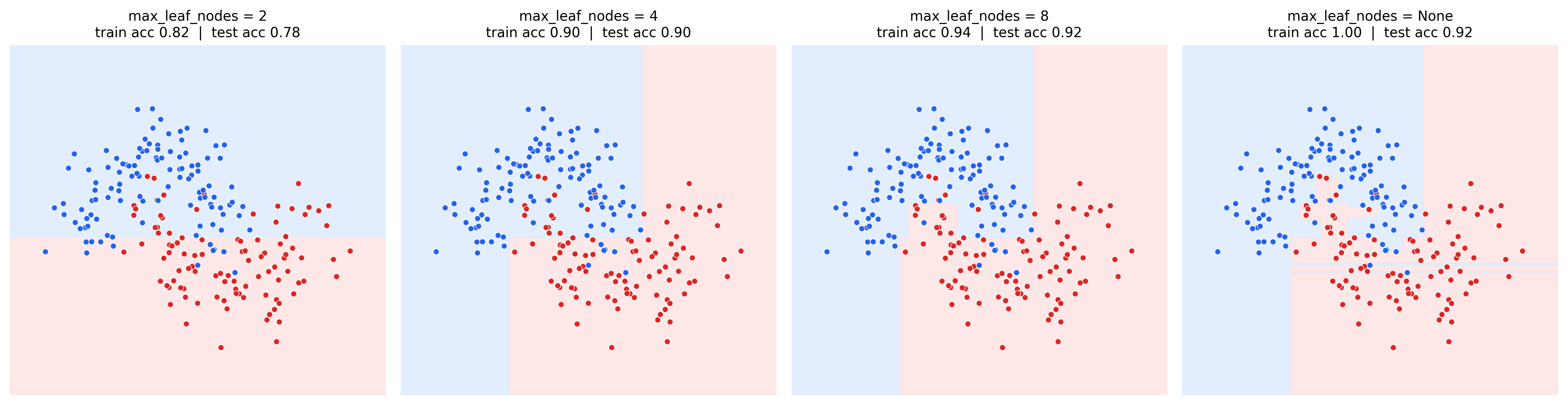
Two leaves means the tree got exactly one split to work with (train 0.82, test 0.78). Each doubling buys a noticeably better fit to the moon shapes, four leaves reaches 0.90/0.90, eight leaves reaches 0.94/0.92, until an unrestricted budget eventually reproduces the same small-islands overfitting seen with unrestricted max_depth (train 1.00, test 0.92). Same shape of trade-off as every hyperparameter so far, just controlling a different structural property of the tree.

8. min_impurity_decrease

Instead of budgeting size, this sets a minimum bar on split quality: a split only happens if it reduces weighted impurity by at least this amount. A node where the best available split barely helps (the classes are already nearly separated, or the split would only isolate a couple of noisy points) gets left as a leaf instead of split further. Set it too high and the tree stops early even where a real pattern remained to be found, underfitting; set it too low (the default, 0.0) and the tree accepts splits that only marginally help, one step short of what min_samples_leaf and max_depth are already there to prevent.

9. Tuning in Practice

None of these hyperparameters has a universally correct value, they're all found the same way: fit with a candidate value, compare train accuracy against test accuracy, and adjust. A large gap (high train, low test) means overfitting, tighten a constraint. Both scores low and close together means underfitting, loosen one. The mental model that ties every hyperparameter in this post together is the same one: more freedom to split (max_depth, max_leaf_nodes unrestricted, min_samples_leaf at 1, min_impurity_decrease at 0) pushes toward overfitting, and tighter limits on any of them push back toward underfitting, until train and test accuracy land close together.