Ch.32: Support Vector Machines, the Maximum Margin Intuition

Inspired by: YouTube

This series moves on to a new algorithm: the Support Vector Machine (SVM). Like K-Nearest Neighbors, it's used for classification (and, as later posts cover, regression too), but its core idea is entirely different: instead of voting among neighbors, SVM asks a geometric question about where exactly to draw the boundary.

1. Two Lines, Both Correct, Not Equally Good

Take a small dataset with two classes, cleanly separable by a straight line. Draw two different candidate separating lines, $\pi_1$ and $\pi_2$, both of which classify every training point correctly:

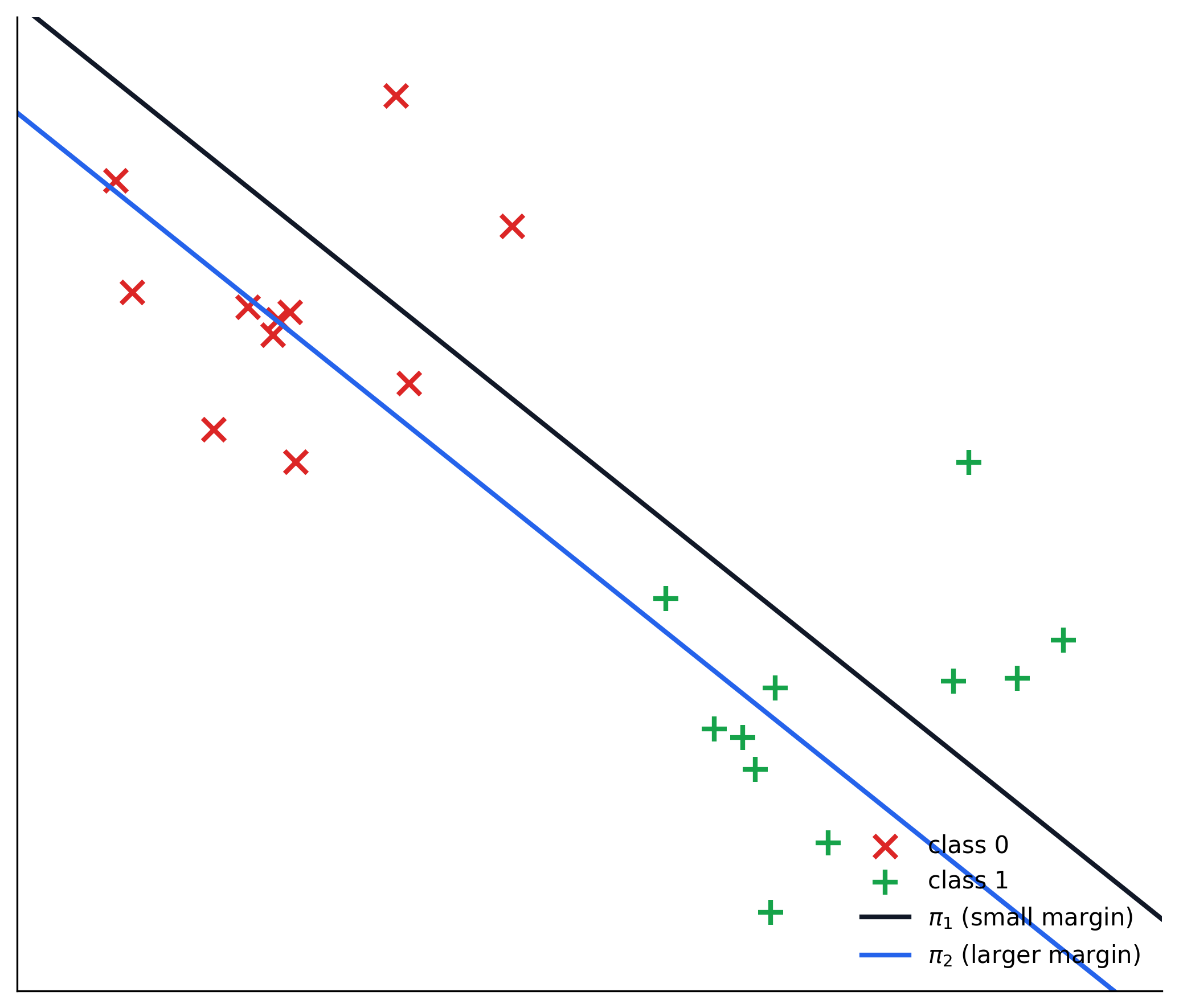
Both lines get 100% training accuracy, so accuracy alone can't say which is better. But $\pi_1$ hugs the red cluster closely, leaving almost no breathing room on that side, while $\pi_2$ sits with a comfortable gap from both classes. Intuitively, $\pi_2$ feels like the safer choice: a new point that lands slightly off from where its class usually sits is far more likely to cross $\pi_1$ than to cross $\pi_2$. That gap is called the margin, and SVM's entire strategy is built around maximizing it.

2. Margin and Prediction Confidence

There's a second way to see why a wider margin matters, connecting straight back to Logistic Regression's sigmoid. Any linear classifier computes a raw score $z = w^Tx + b$ for a point, and a point's distance from the boundary is directly reflected in $z$: points near the line have $z$ close to 0, points far from the line have $z$ far from 0 in either direction. Feeding that score through sigmoid, $\sigma(z) = P(y=1)$, a point near the boundary gets a probability near 0.5, a genuine coin flip, while a point far from the boundary gets a probability confidently close to 0 or 1.

A line placed with a narrow margin, like $\pi_1$, leaves many correctly-classified points sitting uncomfortably close to the boundary, technically right, but with low confidence. A line placed with a wide margin pushes more points further from the boundary, into the confidently-correct zone. Maximizing the margin isn't just about being extra safe against new data, it directly means making more confident predictions on the data already at hand.

3. Building the Margin, Geometrically

The video's whiteboard construction makes "margin" completely concrete: start from a separating line, then slide it in parallel toward the positive class until it just touches the first point in its way. Do the same sliding it toward the negative class. The distance between these two parallel touching lines is the margin, call it $d$. SVM's objective, stated plainly, is: find the separating line that maximizes $d$.

4. Support Vectors

The specific points that the two shifted lines end up touching have a name: support vectors. Fitting an actual linear SVM to the same dataset and marking them:

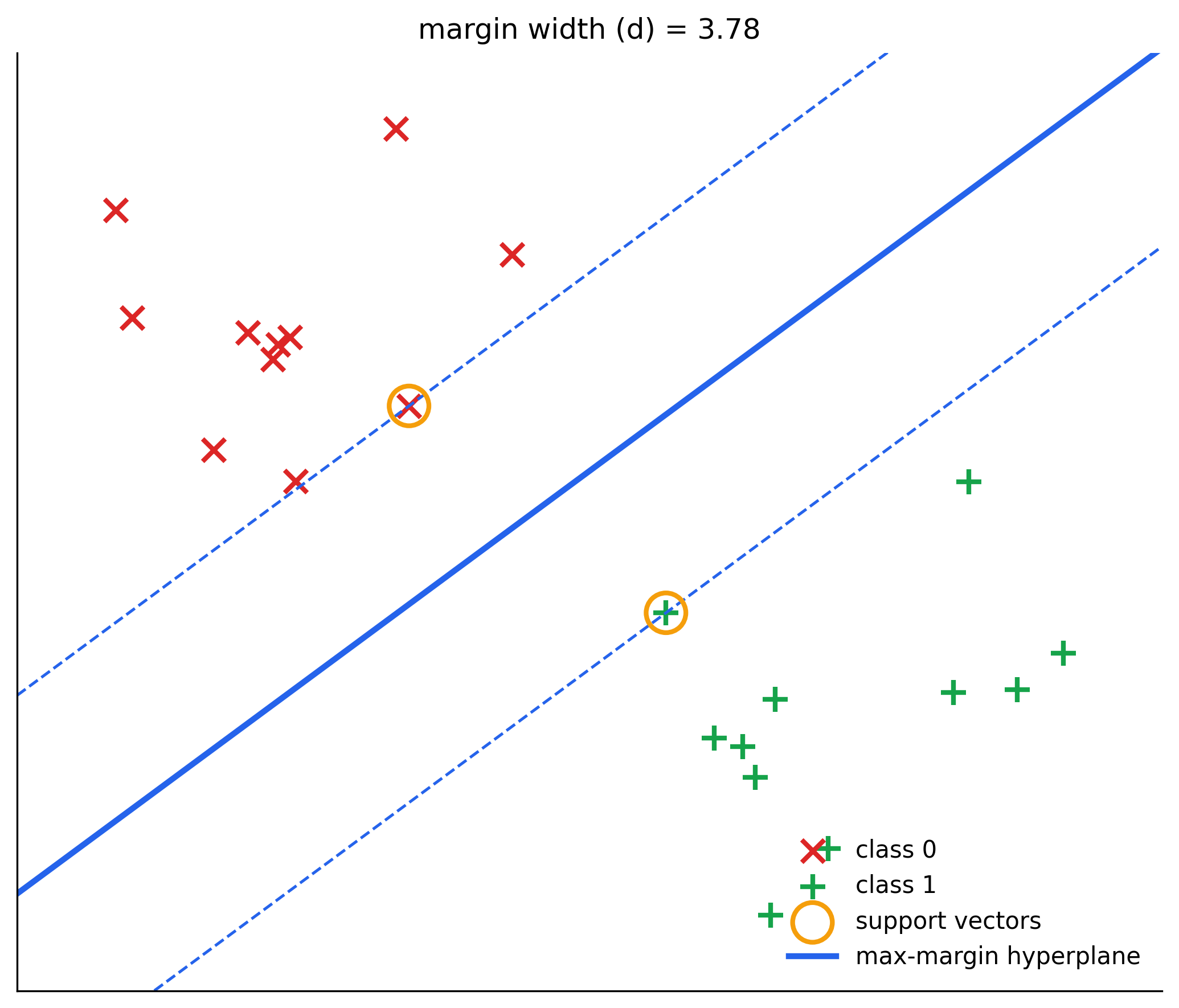
Only two points here are circled as support vectors, one from each class, and they're the sole reason the boundary sits exactly where it does. Every other point could be moved around freely, as long as it doesn't cross into the margin, without changing the fitted line at all. That's a real structural difference from something like Logistic Regression, where every training point pulls on the fitted line through gradient descent; an SVM's boundary is decided entirely by whichever handful of points happen to sit closest to the other class.

5. Where SVM Holds Up Well, and Where It Doesn't

Because the boundary depends only on the support vectors, an outlier that lands deep inside its own class's territory has literally zero effect on the fitted line, it's nowhere near being a support vector. That's a genuine strength over methods where every point has some pull on the result.

The flip side is worth being honest about: an outlier that lands close to or across the other class's territory is exactly the hard case, a single such point can force the margin to shrink drastically, or make the classes impossible to separate with a straight line at all. The fix for that (a "soft" margin that tolerates a few points inside it, controlled by a tunable parameter) is a refinement for a future post, not something this introduction derives.

6. Past a Straight Line

Two more capabilities worth flagging without deriving them here, both explicitly deferred to future posts in this series:

• Non-linear data: SVM isn't limited to data a straight line can separate. The kernel trick projects data into a higher-dimensional space where a linear separator does exist, without ever explicitly computing that higher-dimensional representation. That's a substantial enough idea to earn its own post.
• Beyond binary classification: the same margin-maximizing idea extends to regression (Support Vector Regression) as well as classification, not just the two-class case covered here.

For now, the core idea to hold onto is this: among every line that separates the training data correctly, SVM doesn't stop at "correct," it specifically looks for the one with the most breathing room on both sides, and that choice is entirely determined by the handful of closest points, the support vectors, that give the algorithm its name.