
Ch.11: Polynomial Regression
Inspired by: YouTube
Throughout the previous posts in this series, every regression model we built shared one foundational assumption: the target variable holds a strictly linear relationship with the input features . In simple linear regression (Ch.1), we fitted a straight line . In multiple linear regression (Ch.5), we fitted a flat hyperplane .
Real-world data rarely stays straight. Salary growth vs experience eventually plateaus, crop yield vs fertilizer usage peaks before declining due to soil toxicity, and epidemic spread initially accelerates quadratically before saturating.
When you fit a straight line to naturally curved data, the model fails to capture the true underlying pattern. But does non-linear data require throwing away linear regression entirely and switching to complex non-parametric algorithms?
The answer is no. By applying a feature transformation trick, we can use standard linear regression to fit smooth polynomial curves. This approach is called Polynomial Regression.
Why Polynomial Regression is STILL Linear Regression
A common point of confusion for engineers learning polynomial regression is the name itself. If the model outputs a quadratic curve like , why is it still called Linear Regression?
The distinction lies in what "linear" means in machine learning:
A regression model is defined as linear if it is linear in its parameters (the coefficients ), regardless of whether it is non-linear in its input features .
Consider a polynomial equation with a single input feature :
While the terms are non-linear transformations of , notice how the parameters enter the equation. None of the coefficients are squared (), exponentiated (), multiplied together (), or passed into a trigonometric function (). Every coefficient enters as a simple scalar multiplier in a linear combination.
If we define a set of derived features:
We can rewrite the polynomial equation as:
This equation is mathematically identical to Multiple Linear Regression on the transformed feature vector .
Because the algorithm treats as independent input columns, every OLS closed-form solver and every gradient descent variant (Batch GD, SGD, Mini-Batch GD) works without altering a single line of code.
Step 1: The Non-Linear Data Problem
To see where plain linear regression fails, let us generate a synthetic quadratic dataset using the same parameters as the source notebook:
Where is uniformly sampled between and , and Gaussian noise is added to simulate real-world scatter.
import numpy as np
import matplotlib.pyplot as plt
from sklearn.model_selection import train_test_split
from sklearn.linear_model import LinearRegression
from sklearn.metrics import r2_score

# 1. Generate non-linear quadratic data
np.random.seed(2)
X = 6 * np.random.rand(200, 1) - 3
y = 0.8 * X**2 + 0.9 * X + 2 + np.random.randn(200, 1)

# 2. Train-test split
X_train, X_test, y_train, y_test = train_test_split(X, y, test_size=0.2, random_state=2)

# 3. Fit plain Linear Regression
lr = LinearRegression()
lr.fit(X_train, y_train)

# 4. Evaluate R2 score on test set
y_pred = lr.predict(X_test)
print("Test R2 Score:", r2_score(y_test, y_pred))
# Output: ~0.53
When we fit a standard linear regression model directly to , the model tries to force a straight line through a parabolic distribution:
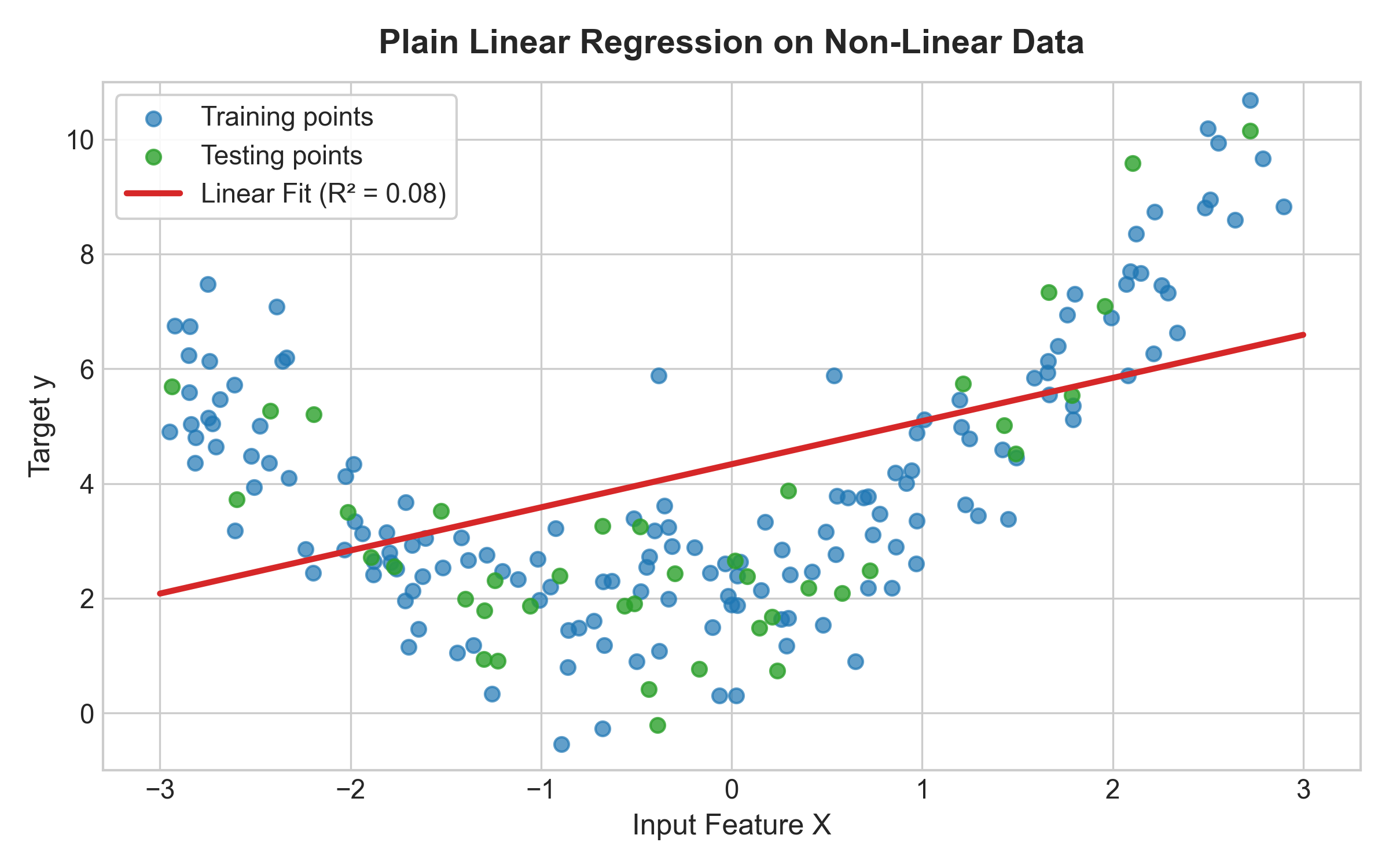
The straight line gets an score of only . It completely cuts through the middle of the parabola, systematically overestimating in the center range () and underestimating at the extremes ( or ).
Step 2: Feature Transformation with PolynomialFeatures
To allow our linear model to fit a curve, we must expand the input feature matrix from 1 dimension () to 2 dimensions ().
scikit-learn provides the PolynomialFeatures class inside sklearn.preprocessing specifically for this task:
from sklearn.preprocessing import PolynomialFeatures

# Create PolynomialFeatures transformer for degree 2
poly = PolynomialFeatures(degree=2, include_bias=True)

# Transform training and testing feature arrays
X_train_trans = poly.fit_transform(X_train)
X_test_trans = poly.transform(X_test)

print("Original shape:", X_train.shape)
print("Transformed shape:", X_train_trans.shape)
# Output:
# Original shape: (160, 1)
# Transformed shape: (160, 3)
Let us look at a single raw input sample and its transformed representation:
print("Raw input X_train[0]:", X_train[0])
print("Transformed X_train_trans[0]:", X_train_trans[0])
# Output (example value x = 0.441):
# Raw input X_train[0]: [0.441142]
# Transformed X_train_trans[0]: [1.0, 0.441142, 0.194606]
The include_bias Parameter
Notice that PolynomialFeatures(degree=2, include_bias=True) outputs 3 columns for a single input :
- Column 0: (the bias / intercept term)
- Column 1: (the original feature)
- Column 2: (the squared feature)
That leading column of 1.0s is there because a linear model's prediction looks like . The term needs something to multiply, so include_bias=True manufactures a constant feature (always ) for it to attach to. This is the same trick used for the augmented matrix in plain linear regression, PolynomialFeatures is just generating it automatically alongside the polynomial terms.
The catch is that LinearRegression already does this for you: by default fit_intercept=True, so it fits its own intercept internally without needing an explicit column of ones. If you feed it a matrix that already has one (from include_bias=True), you end up with two things both trying to represent the intercept, one from the transformer's bias column, one from LinearRegression's own fit_intercept. This does not break the fit (the two collapse into an equivalent solution), but it is redundant and wastes a column.
The practical rule: when your transformed features feed straight into LinearRegression, set include_bias=False and let LinearRegression handle the intercept on its own. Only set include_bias=True if you are handing the features to something that does not fit its own intercept, in which case you need to supply that constant column yourself.
Step 3: Fitting Linear Regression on Transformed Features
Now that X_train_trans contains , we pass it into standard LinearRegression:
# Fit LinearRegression on transformed polynomial features
lr_poly = LinearRegression()
lr_poly.fit(X_train_trans, y_train)

# Evaluate on transformed test features
y_pred_poly = lr_poly.predict(X_test_trans)
print("Polynomial Regressor R2 Score:", r2_score(y_test, y_pred_poly))
# Output: ~0.82
The score jumps from up to . Plotting the predictions reveals how well the fitted model captures the parabolic shape:
# Plot fitted polynomial curve
X_new = np.linspace(-3, 3, 200).reshape(200, 1)
X_new_poly = poly.transform(X_new)
y_new = lr_poly.predict(X_new_poly)

plt.plot(X_new, y_new, "r-", linewidth=2.5, label="Predictions")
plt.plot(X_train, y_train, "b.", label="Training points")
plt.plot(X_test, y_test, "g.", label="Testing points")
plt.xlabel("X")
plt.ylabel("y")
plt.legend()
plt.show()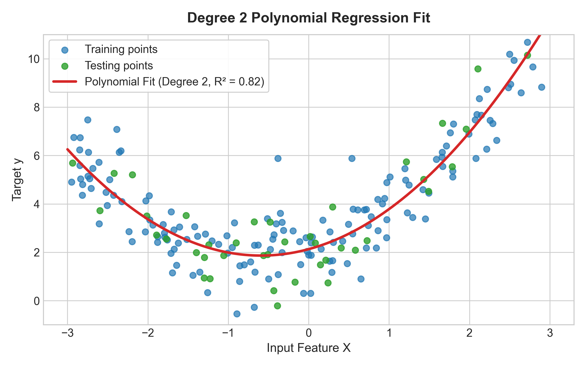
Inspecting Model Coefficients vs Ground Truth
Since we generated the synthetic data using , let us inspect the coefficients learned by lr_poly:
print("Coefficients (lr_poly.coef_):", lr_poly.coef_)
print("Intercept (lr_poly.intercept_):", lr_poly.intercept_)
# Output:
# Coefficients: [[0.         0.89201556 0.78543881]]
# Intercept: [1.94823058]
Matching each coefficient to its feature:
- Intercept (): (True value: )
- Linear term ( for ): (True value: )
- Quadratic term ( for ): (True value: )
The learned model equation is . The slight discrepancy between estimated parameters and ground truth comes entirely from the random noise added during data creation.
Gradient Descent with Polynomial Features
Because polynomial regression is simply linear regression on transformed columns, we can also use iterative optimizers like SGDRegressor or Mini-Batch GD (from Ch.10):
from sklearn.linear_model import SGDRegressor

# Apply Stochastic Gradient Descent on transformed features
sgd = SGDRegressor(max_iter=1000, tol=1e-3, random_state=42)
sgd.fit(X_train_trans, y_train.ravel())

y_pred_sgd = sgd.predict(X_test_trans)
print("SGD Polynomial R2 Score:", r2_score(y_test, y_pred_sgd))
Important Note on Scaling: When using high-degree polynomial features with gradient descent, feature scaling is mandatory. Because grows rapidly (), unscaled higher-order features create ill-conditioned loss surfaces, causing gradient descent to oscillate wildly or diverge unless features are passed through
StandardScaler.
The Degree Trade-off: Underfitting vs. Overfitting
The degree hyperparameter controls the maximum exponent used in the transformation. Choosing the right degree is critical:
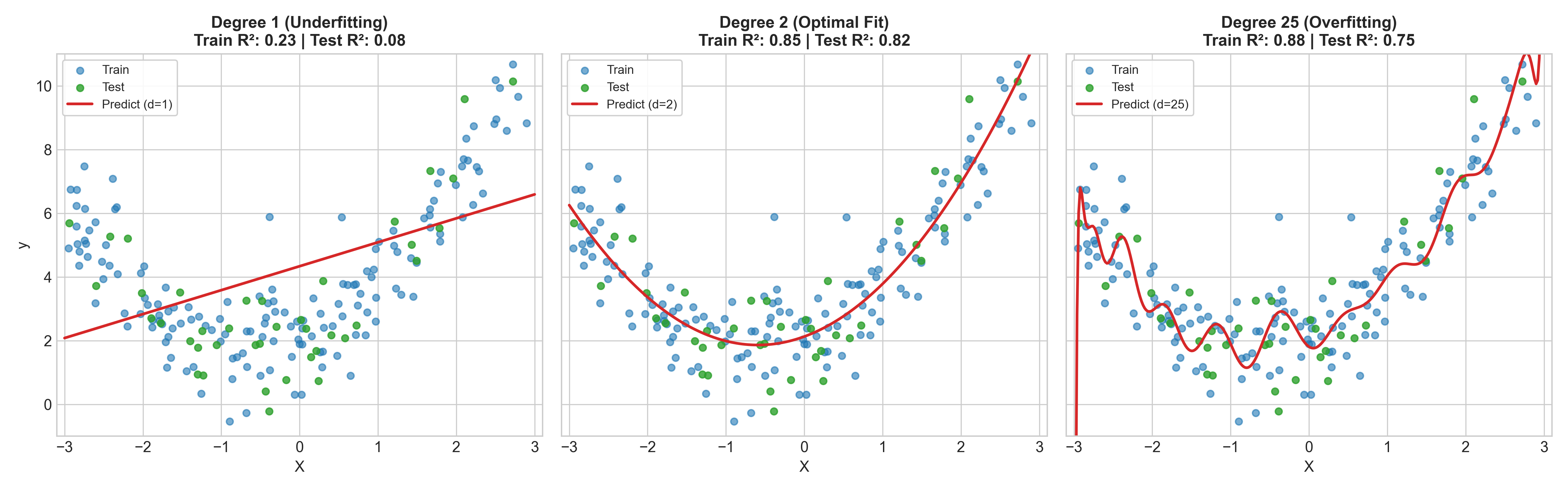
- Degree 1 (Underfitting / High Bias): The model is constrained to a straight line . It lacks the capacity to capture curvature, leading to high error on both training and test data.
- Degree 2 (Optimal Fit / Balanced): Matches the true quadratic nature of the data. It captures curvature while ignoring random noise fluctuations.
- Degree 25+ (Overfitting / High Variance): A degree 25 polynomial has 25 flexible parameters. Instead of learning the smooth parabolic trend, the curve oscillates violently to pass directly through individual noise points in the training set.
Why High-Degree Polynomials Overfit
When degree is set to 25, the model attempts to minimize training MSE by bending its curve sharply between adjacent training samples.
While the training score approaches , the test score collapses into negative territory (e.g., ). The model completely loses its ability to generalize to new, unseen data points.
In scikit-learn, building high-degree polynomial pipelines is best handled using Pipeline:
from sklearn.pipeline import Pipeline
from sklearn.preprocessing import StandardScaler

def fit_polynomial_pipeline(degree):
    model = Pipeline([
        ('poly_features', PolynomialFeatures(degree=degree, include_bias=False)),
        ('std_scaler', StandardScaler()),
        ('lin_reg', LinearRegression())
    ])
    model.fit(X_train, y_train)
    return model
Multiple Feature Polynomial Regression (Higher Dimensions)
What happens when our dataset contains more than one input feature?
Suppose we have two input features and . Applying PolynomialFeatures(degree=2) generates 6 features:
Notice the middle term . This is an interaction term. Polynomial regression automatically creates interaction terms between features, allowing the model to capture dependencies where the effect of on depends on the current value of .
Why is NOT Included in Degree 2
A common question is: why does
PolynomialFeatures(degree=2)include , but not ?In algebra, the degree of a monomial is defined as the sum of its exponents:
For
degree=2, the constraint is :
- Term : degree
- Term : degree
- Term : degree (excluded)
The Combinatorial Explosion of Features
For input features and degree , the total number of output features generated by PolynomialFeatures (including bias) is given by the combination formula:
As either or grows, the feature count explodes exponentially:
| Input Features () | Degree () | Output Features () |
|---|---|---|
| 1 | 2 | 3 |
| 2 | 2 | 6 |
| 5 | 3 | 56 |
| 10 | 4 | 1,001 |
| 20 | 5 | 53,130 |
With 20 features and degree 5, a dataset with only 1,000 rows explodes into 53,130 features, instantly triggering severe overfitting and massive memory consumption.
Visualizing 3D Polynomial Regression
When we fit polynomial regression on 2 features predicting target , plain multiple linear regression fits a flat 2D plane:
Polynomial regression of degree 2 fits a curved 3D surface (a paraboloid):
As seen in the 3D plot above, while the flat plane cuts arbitrarily through the bowl-shaped data distribution, the degree 2 polynomial surface curves upward smoothly, capturing the true 3D curvature of the dataset.
Summary & Key Takeaways
- Linear in Parameters: Polynomial regression fits curved lines using standard linear regression because the model equation remains linear with respect to its coefficients .
- Feature Transformation:
PolynomialFeatures(degree=d)transforms input vector into higher-order powers and cross-product interaction terms. - Hyperparameter Selection: Degree 1 underfits (high bias); excessively high degrees overfit (high variance).
- Combinatorial Explosion: The feature count grows as . For high-dimensional datasets (), high polynomial degrees quickly become computationally unfeasible and prone to extreme overfitting.
- Preprocessing: Always scale features with
StandardScalerwhen applying gradient descent or regularization to polynomial features.
In the next post, we will explore regularization techniques (Ridge, Lasso, and ElasticNet) to prevent high-degree polynomial models from overfitting.