Ch.16: Five Things to Know About Ridge Regression

Inspired by: YouTube

The last three posts built up Ridge Regression from the loss function (Ch.13) through its closed-form and gradient descent solutions (Ch.14, Ch.15). This post closes out the topic with five intuitions that tend to come up as interview questions once someone knows Ridge exists but hasn't sat with how $\lambda$ actually behaves.

1. Coefficients Shrink Toward Zero, But Never Reach It

Ridge's loss is $\sum (y_i - \hat y_i)^2 + \lambda \sum w_j^2$. At $\lambda = 0$ it's plain OLS. As $\lambda \to \infty$, every coefficient gets pulled toward zero, but never all the way there.

from sklearn.datasets import load_diabetes
from sklearn.model_selection import train_test_split
from sklearn.linear_model import Ridge
from sklearn.metrics import r2_score
 
data = load_diabetes()
X_train, X_test, y_train, y_test = train_test_split(data.data, data.target, test_size=0.2, random_state=2)
 
coefs, r2_scores = [], []
for alpha in [0, 10, 100, 1000]:
    reg = Ridge(alpha=alpha)
    reg.fit(X_train, y_train)
    coefs.append(reg.coef_.tolist())
    r2_scores.append(r2_score(y_test, reg.predict(X_test)))
 
print([round(r, 2) for r in r2_scores])
# [0.44, 0.15, 0.01, -0.01]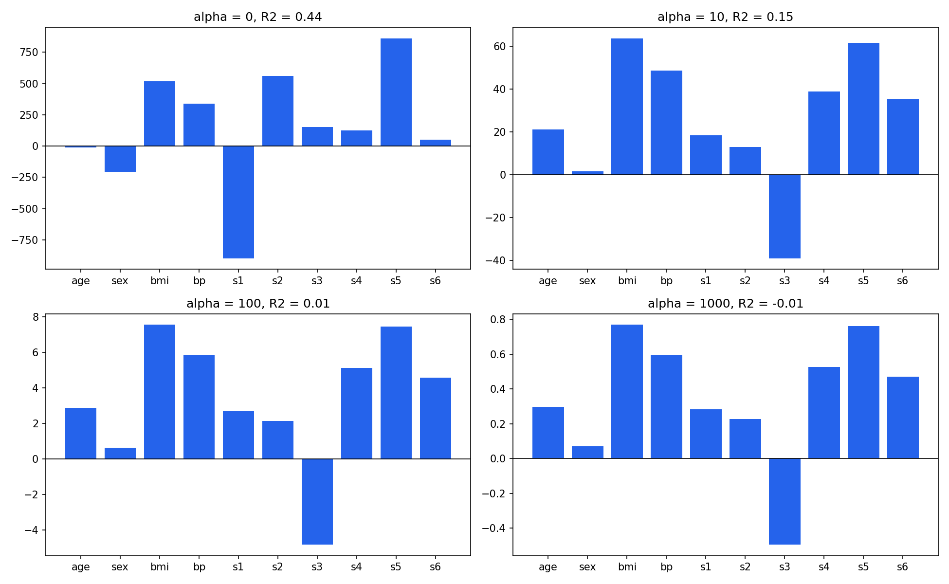

At alpha=0 the bars span roughly -900 to 900. By alpha=1000 every bar has collapsed to a sliver near zero, and $R^2$ has dropped from 0.44 to -0.01, the model has been regularized into predicting close to the mean. Note the $R^2$ dropping this far isn't Ridge failing, it's alpha=1000 being a wildly oversized penalty for a 10-feature dataset; the point is only to make the shrinkage-toward-zero-without-reaching-it visible at an exaggerated scale. None of the ten features' bars ever touch the black zero line exactly, at any alpha. That's the core distinction between Ridge (L2) and Lasso (L1) regression: Ridge shrinks, Lasso can zero out.

2. Larger Coefficients Shrink Faster

Not every coefficient shrinks at the same rate. A coefficient that starts large drops proportionally faster than one that starts small.

alphas = [0, 0.0001, 0.0005, 0.001, 0.005, 0.1, 0.5, 1, 5, 10]
coefs = []
for alpha in alphas:
    reg = Ridge(alpha=alpha)
    reg.fit(X_train, y_train)
    coefs.append(reg.coef_.tolist())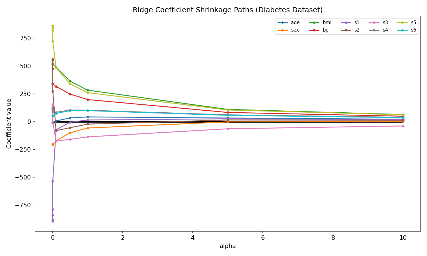

s5 starts at 861 and by alpha=10 has fallen to 62, a drop of roughly 93%. s1 starts at -895 and lands near 18. Meanwhile a feature that starts small, like sex at roughly -206, still shrinks, but nowhere near as steeply in absolute terms. The intuition: the penalty term is $\lambda w_j^2$, so a coefficient's contribution to the loss grows quadratically with its own size, which means the gradient pulling it down is also proportionally larger. Big coefficients have more to lose.

3. Alpha Controls the Bias-Variance Tradeoff

Ch.12 covered bias and variance in general. Ridge's $\lambda$ is a direct dial on that tradeoff: alpha=0 lets a model overfit freely (low bias, high variance), and pushing alpha up trades variance for bias until the model underfits (high bias, low variance).

import numpy as np
from sklearn.preprocessing import PolynomialFeatures
from mlxtend.evaluate import bias_variance_decomp
 
np.random.seed(2)
m = 100
X = 5 * np.random.rand(m, 1) - 2
y = 0.7 * X ** 2 - 2 * X + 3 + np.random.randn(m, 1)
 
X_train, X_test, y_train, y_test = train_test_split(X.reshape(100, 1), y.reshape(100), test_size=0.2, random_state=2)
 
poly = PolynomialFeatures(degree=15)
X_train_p = poly.fit_transform(X_train)
X_test_p = poly.transform(X_test)
 
alphas = np.linspace(0, 30, 60)
loss, bias, variance = [], [], []
for alpha in alphas:
    reg = Ridge(alpha=alpha)
    avg_loss, avg_bias, avg_var = bias_variance_decomp(
        reg, X_train_p, y_train, X_test_p, y_test, loss='mse', random_seed=123)
    loss.append(avg_loss)
    bias.append(avg_bias)
    variance.append(avg_var)

A degree-15 polynomial is deliberately overkill for this quadratic-shaped data, which is exactly what makes the tradeoff visible: at low alpha it has enough freedom to chase noise. mlxtend.evaluate.bias_variance_decomp fits the model repeatedly on resampled training sets and decomposes the average test error into bias and variance:

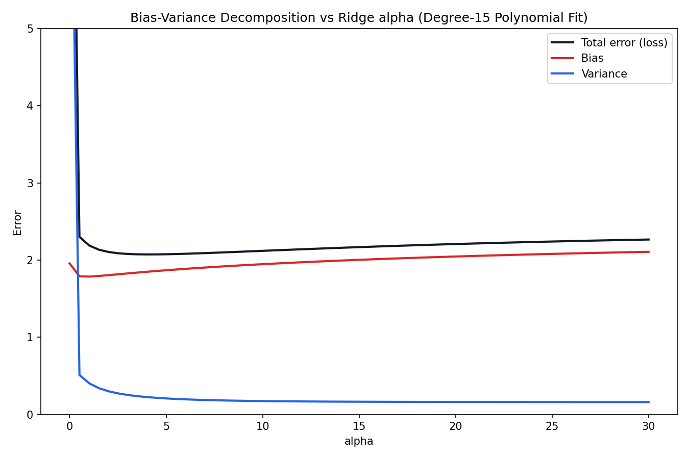
At alpha=0, variance is high (the degree-15 fit is chasing every data point) and bias is low. As alpha climbs, variance falls and bias rises, the opposite trends the theory predicts. Total loss (the black line) traces a U-shape with the minimum near alpha≈4.1, right around where the bias and variance curves cross. That crossing point, not alpha=0 and not some very large alpha, is where the sweet spot lives: enough regularization to tame variance, not so much that bias takes over.

4. Alpha Reshapes the Loss Surface

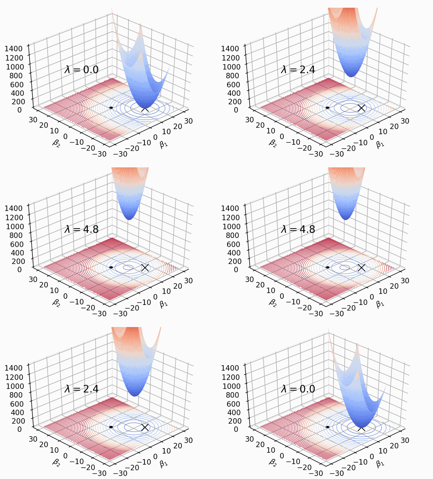
Increasing $\lambda$ doesn't just change where the loss is minimized, it changes the shape of the loss curve itself, lifting it and dragging its minimum toward the origin.

from sklearn.datasets import make_regression
from sklearn.linear_model import LinearRegression
 
X, y = make_regression(n_samples=100, n_features=1, n_informative=1, n_targets=1, noise=20, random_state=13)
 
reg = LinearRegression()
reg.fit(X, y)
print(reg.coef_, reg.intercept_)
# [27.83] -2.29
 
def cal_loss(m, alpha):
    return np.sum((y - m * X.ravel() + 2.29) ** 2) + alpha * m * m
 
m = np.linspace(-45, 100, 200)
for alpha in [0, 10, 20, 30, 40, 50, 100]:
    loss = [cal_loss(mi, alpha) for mi in m]
    # plot m against loss for each alpha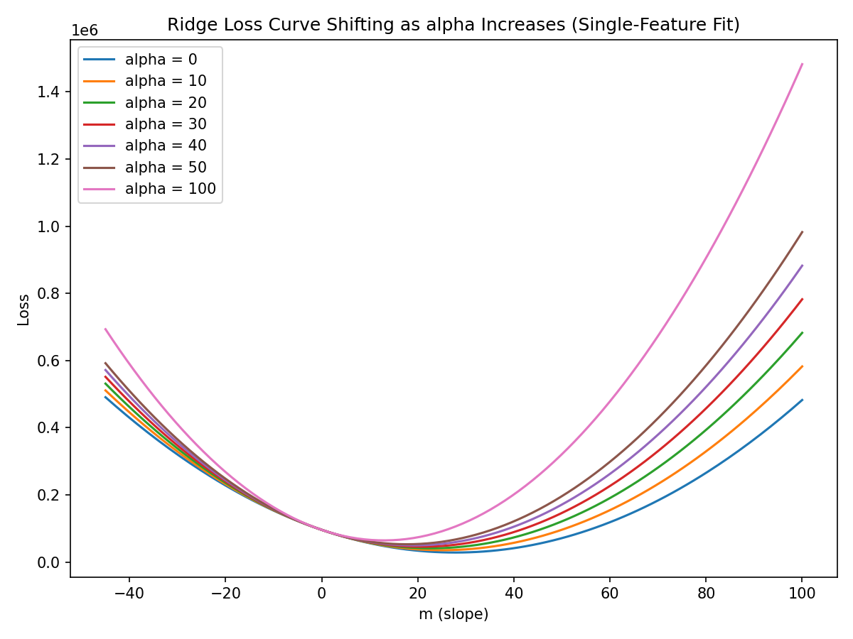

At alpha=0 the parabola's minimum sits at m≈27.86, matching LinearRegression's unregularized coefficient. As alpha climbs to 10, 20, up through 100, each new parabola is narrower and its minimum has shifted further left, toward m≈13.29 at alpha=100. The $\lambda m^2$ term added to the loss grows quadratically as $m$ moves away from zero, so it increasingly penalizes staying at the old minimum, which drags the whole curve's low point back toward the origin. This is the same shrinkage from point 1, just viewed as a moving minimum instead of a moving coefficient value.

With two coefficients, the loss is a literal 3D bowl (a paraboloid) instead of a 2D parabola, exactly what the video plots and animates over $(w_1, w_2)$:

from sklearn.datasets import make_regression
 
X, y = make_regression(n_samples=100, n_features=2, n_informative=2, n_targets=1, noise=15, random_state=13)
 
def loss(w1, w2, alpha):
    W = np.stack([w1.ravel(), w2.ravel()], axis=0)
    resid = y[:, None] - X @ W
    data_loss = np.sum(resid ** 2, axis=0)
    reg_loss = alpha * (w1.ravel() ** 2 + w2.ravel() ** 2)
    return (data_loss + reg_loss).reshape(w1.shape)
 
w1 = np.linspace(-20, 100, 140)
w2 = np.linspace(-20, 100, 140)
W1, W2 = np.meshgrid(w1, w2)
 
Z = loss(W1, W2, alpha)  # plot_surface(W1, W2, Z) in 3D, mark the minimum

Rather than a fixed set of alpha snapshots, drag the slider below to move alpha continuously and watch the bowl's minimum, the red dot, respond in real time. It's the same quadratic form: w1 and w2 steer along $X^TX$, and the readout above the plot always shows the current alpha and the minimum's coordinates together, so there's no need to scroll between a screenshot's title and its caption to see both at once.

At alpha=0 the bowl is wide and shallow, and its minimum sits at (81.0, 26.1), matching what LinearRegression finds unregularized. Drag the slider up and the walls of the bowl visibly steepen and close in, while the minimum climbs the $w_1$-$w_2$ plane back toward the black diamond at the origin. The two coordinates shrink together and roughly proportionally, since both are pulled by the same $\lambda(w_1^2 + w_2^2)$ term, which is exactly the pattern from points 1 and 2: every coefficient shrinks toward, but never reaches, the origin, with the ones that started furthest out moving the most in absolute terms.

5. Why It's Called "Ridge"

This one's more geometric than algebraic, and comes from viewing Ridge as a constrained optimization problem rather than a penalized one. The two formulations are mathematically equivalent, but the constrained view is where the name comes from.

Instead of adding $\lambda \sum w_j^2$ to the loss directly, imagine minimizing $\sum (y_i - \hat y_i)^2$ subject to a hard constraint: $\sum w_j^2 \le t$ for some fixed budget $t$. With two coefficients $\beta_1, \beta_2$, that constraint is a circle in $(\beta_1, \beta_2)$-space, since $\beta_1^2 + \beta_2^2 \le t$ is exactly the equation of a disk.

Without any constraint, OLS would settle at whatever $(\beta_1, \beta_2)$ minimizes the loss outright. With the constraint in place, the solution is forced to land somewhere on the boundary of that circle, specifically wherever the circle is tangent to the loss function's elliptical contours, the point on the circle's edge closest to the unconstrained OLS solution. Trace that boundary and it looks like a ridge running around the rim of the loss surface, which is where the technique's name comes from: the solution rides the edge of a circular constraint region rather than settling into an unconstrained valley.

A visualization of this from explained.ai shows the constraint circle and the elliptical loss contours shifting together as $\lambda$ changes, with the solution always pinned to the circle's boundary. Working out exactly how the circle's radius maps to $\lambda$, and why an L1 constraint (Lasso) produces a diamond instead of a circle, is enough of its own topic to warrant a separate post later.

6. A Practical Note on When to Use It

Ridge earns its keep when there are enough input features that overfitting and multicollinearity are real risks, roughly two or more, and the benefit grows with feature count. With a single input feature, there's little for L2 regularization to do; it's most useful exactly where OLS is most likely to memorize noise instead of generalizing.

That covers the five recurring questions Ridge tends to draw once someone's past "what is it" and into "how does it actually behave." Next up: Lasso Regression, L1 regularization, which handles all of this differently enough that coefficients really can hit exactly zero.