Ch.17: Lasso Regression: The Intuition

Inspired by: YouTube

Ridge Regression (Ch.13 through Ch.16) adds $\lambda \sum w_j^2$ to the loss, the squared L2 norm of the weight vector. Lasso Regression, also called L1 regularization, makes exactly one change: it penalizes the L1 norm instead.

$L = \sum_{i=1}^n (y_i - \hat y_i)^2 + \lambda \sum_{j=1}^p |w_j|$

Swap the square for an absolute value and every other piece of the loss stays identical. That one-character-sounding change turns out to produce a genuinely different kind of model, one where coefficients don't just shrink toward zero, they can land exactly on it.

1. Coefficients Can Hit Exactly Zero

Start with the same single-feature setup used throughout the Ridge posts:

from sklearn.linear_model import Lasso, LinearRegression
from sklearn.datasets import make_regression
from sklearn.model_selection import train_test_split
 
X, y = make_regression(n_samples=100, n_features=1, n_informative=1, n_targets=1, noise=20, random_state=13)
X_train, X_test, y_train, y_test = train_test_split(X, y, test_size=0.2, random_state=13)
 
reg = LinearRegression()
reg.fit(X_train, y_train)
print(reg.coef_, reg.intercept_)
# [28.68] -2.09

for alpha in [0, 1, 5, 10, 30]:
    L = Lasso(alpha=alpha)
    L.fit(X_train, y_train)
    print(f"alpha={alpha}", L.coef_, L.intercept_)
# alpha=0  [28.68] -2.09
# alpha=1  [27.43] -2.16
# alpha=5  [22.46] -2.43
# alpha=10 [16.25] -2.76
# alpha=30 [0.]    -3.65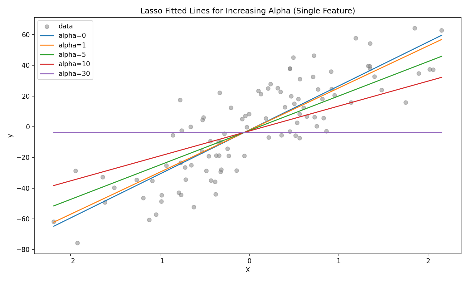

By alpha=30 the coefficient isn't just small, it's exactly 0.0, and the fitted line has gone perfectly flat, predicting the mean of y regardless of X. Recall from Ch.16 that Ridge coefficients shrink toward zero but never reach it, no matter how large alpha gets. This is the single defining difference between the two techniques, and everything else in this post follows from it.

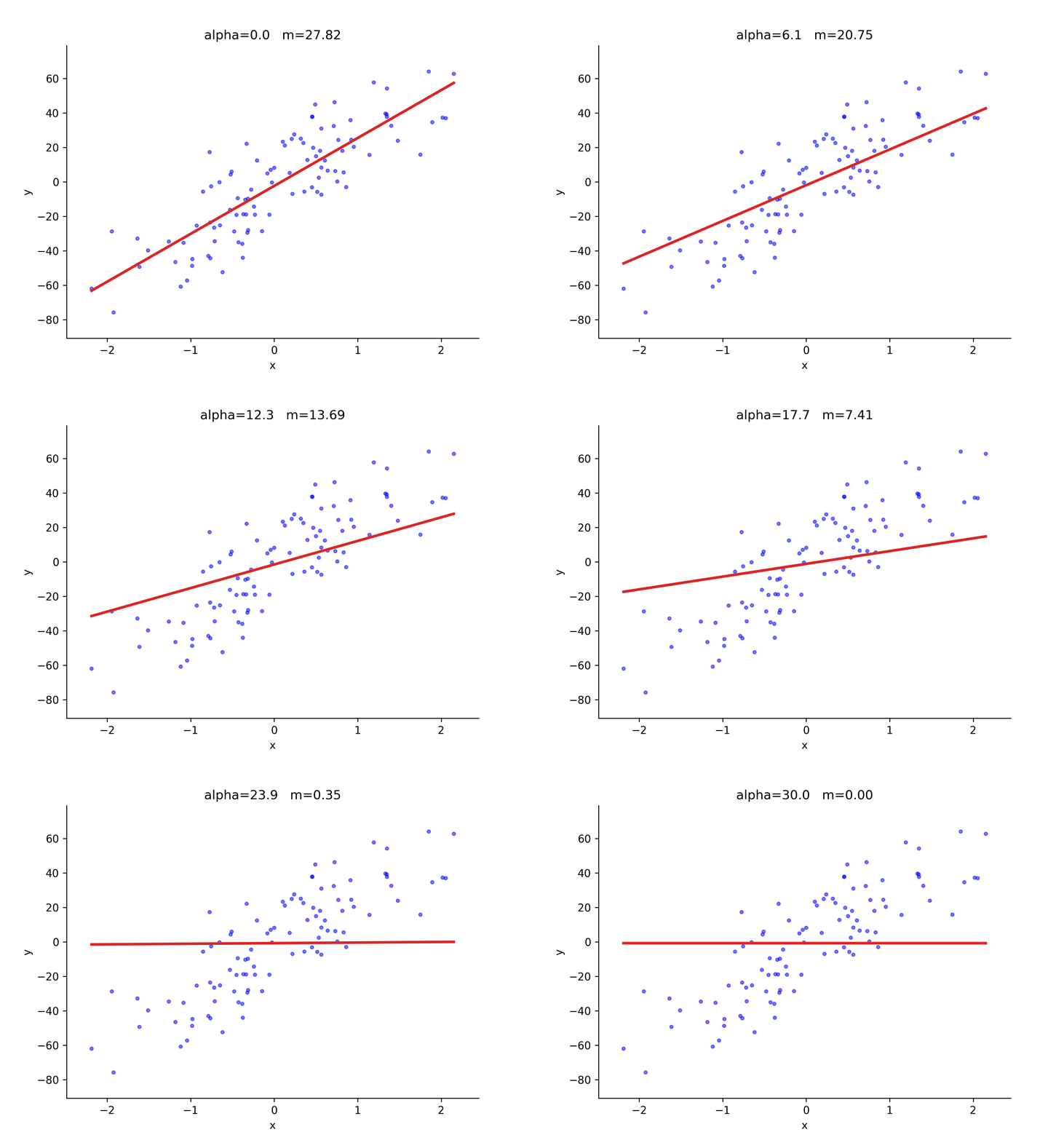
Watching alpha sweep continuously makes the flattening obvious as a single smooth process, not just five snapshots: the line pivots down from its steepest slope toward horizontal, and once it goes flat at alpha=30 it stays pinned there for any alpha beyond that.

2. Same Behavior on a Nonlinear Fit

Fitting a degree-16 polynomial with Lasso on nonlinear data shows the same under/overfitting tradeoff Ridge has, just with sparser coefficients doing the work:

from sklearn.pipeline import Pipeline
from sklearn.preprocessing import PolynomialFeatures
 
def get_preds_lasso(x1, x2, alpha):
    model = Pipeline([
        ('poly_feats', PolynomialFeatures(degree=16)),
        ('lasso', Lasso(alpha=alpha)),
    ])
    model.fit(x1, x2)
    return model.predict(x1)
 
for alpha in [0, 0.1, 1]:
    preds = get_preds_lasso(x1, x2, alpha)
    # plot x1 against preds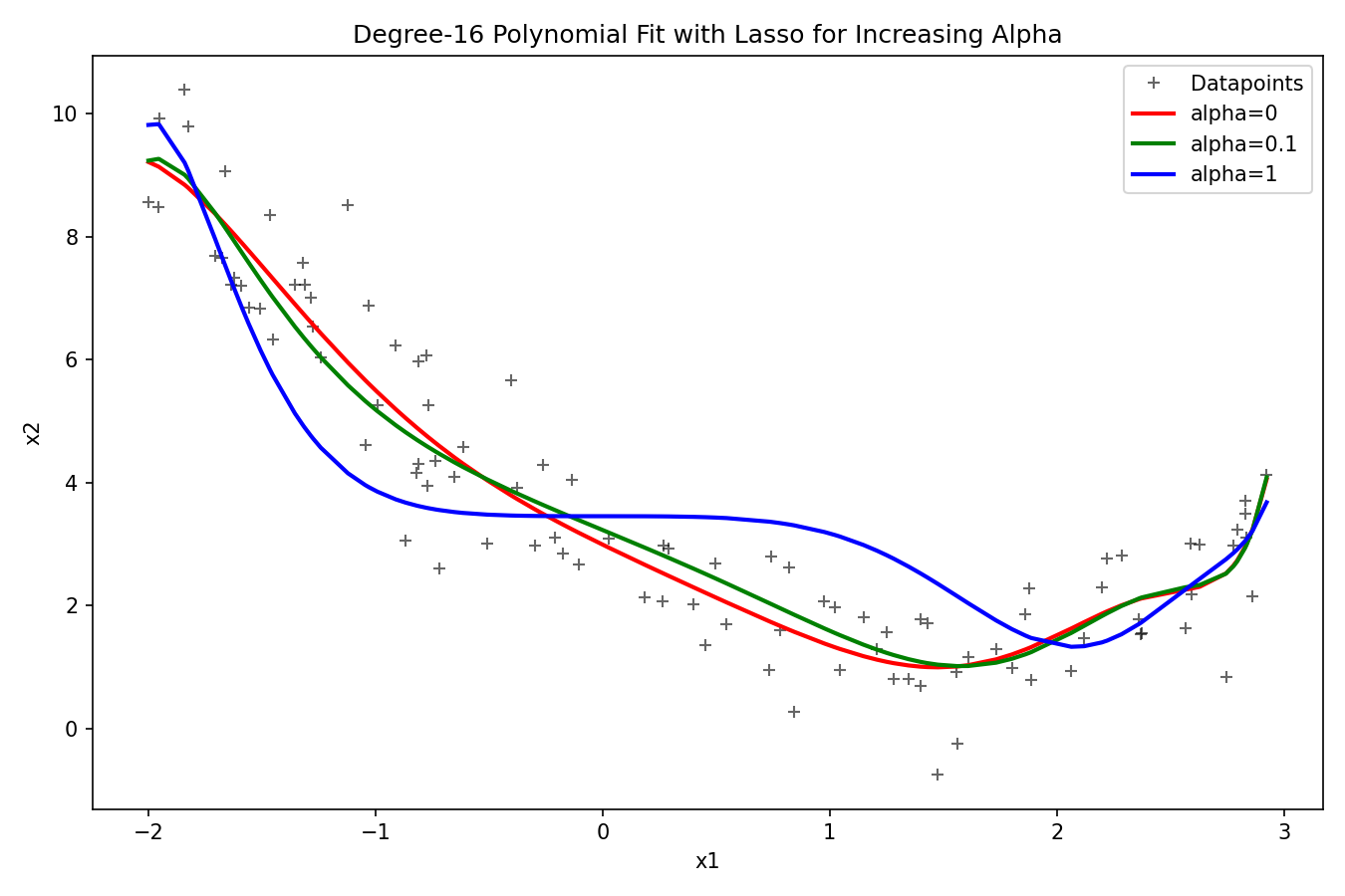

alpha=0 (red) chases the data closely, a textbook overfit. alpha=0.1 (green) smooths that out a little. alpha=1 (blue) smooths it out a lot, sitting close to the true underlying curve without tracking individual points. Same story as Ridge: too little regularization overfits, too much underfits.

3. Automatic Feature Selection

This is where the "coefficients hit exactly zero" property actually pays off. On the diabetes dataset:

from sklearn.datasets import load_diabetes
from sklearn.metrics import r2_score
 
data = load_diabetes()
X_train, X_test, y_train, y_test = train_test_split(data.data, data.target, test_size=0.2, random_state=2)
 
coefs, r2_scores = [], []
for alpha in [0, 0.1, 1, 10]:
    reg = Lasso(alpha=alpha)
    reg.fit(X_train, y_train)
    coefs.append(reg.coef_.tolist())
    r2_scores.append(r2_score(y_test, reg.predict(X_test)))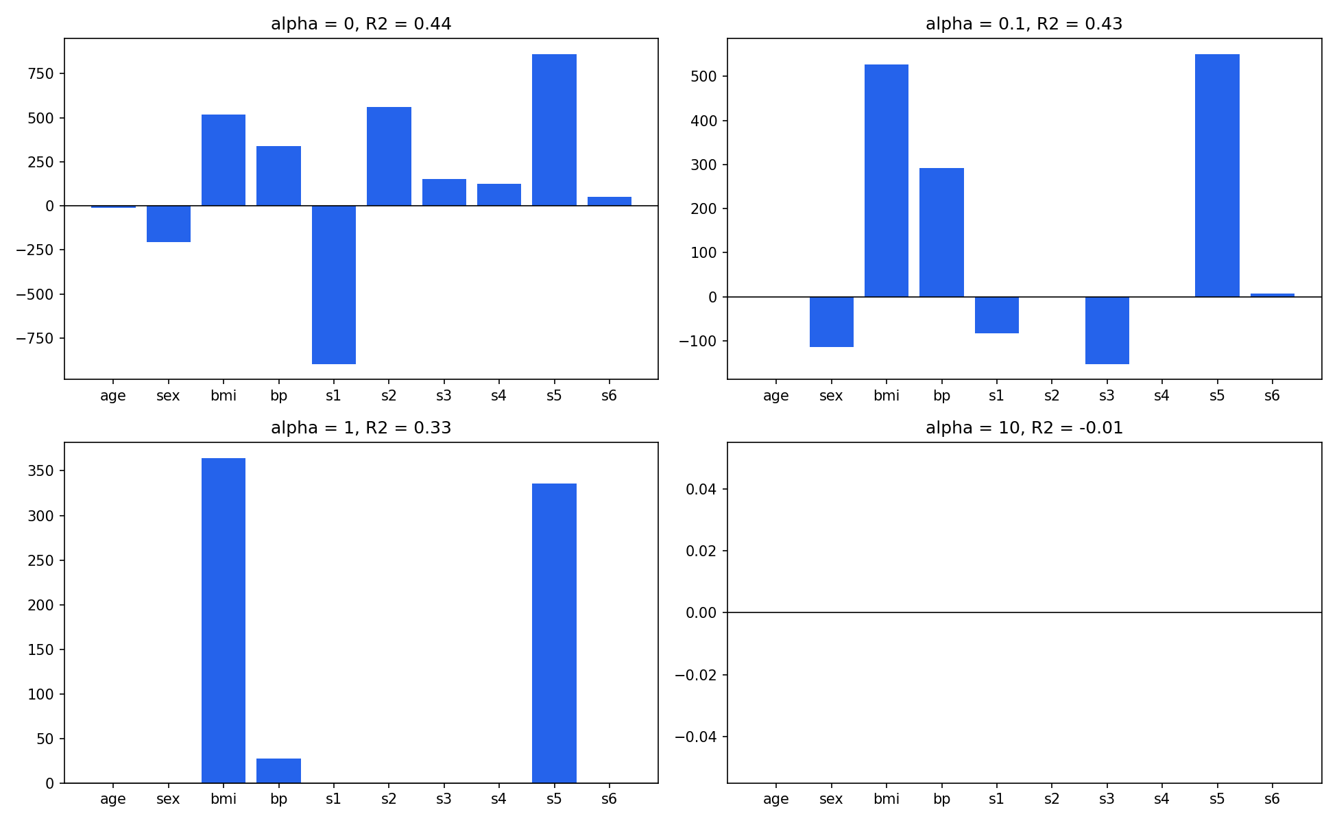

At alpha=0 all ten features have a nonzero coefficient. By alpha=0.1, age, s2, and s4 have dropped to exactly zero, bars that simply aren't there anymore, not just short ones. By alpha=1, only bmi, bp, and s5 survive. By alpha=10, every coefficient is 0.0 and $R^2$ has collapsed to -0.01, the model predicting nothing but the mean.

This is Lasso performing feature selection as a side effect of regularization. A column whose coefficient lands on exactly zero contributes nothing to predictions, so it can be dropped from the dataset entirely with zero change in output. Ridge can tell a column is unimportant too, its coefficient will be small, but it never actually removes the column: some tiny nonzero weight always remains, and the feature still has to be collected, stored, and fed into the model at inference time. For a high-dimensional dataset where many columns genuinely don't matter, that difference decides which algorithm to reach for.

4. Larger Coefficients Still Shrink First, But Now They Also Disappear First

The coefficient paths across a wider alpha range make the order of elimination visible:

alphas = [0.0001, 0.0005, 0.001, 0.005, 0.01, 0.05, 0.1, 0.5, 1, 2, 5, 10]
coefs = []
for alpha in alphas:
    reg = Lasso(alpha=alpha)
    reg.fit(X_train, y_train)
    coefs.append(reg.coef_.tolist())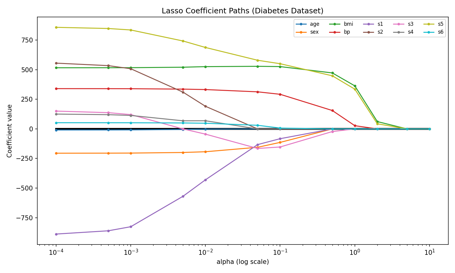

s1 starts around -895 and drops fast in relative terms, down to -132 by alpha=0.05, but doesn't actually hit exactly 0 until somewhere between alpha=0.1 and alpha=0.5. s5 starts around 857, the single largest coefficient, and survives far longer: still 43.5 at alpha=2 before finally being zeroed out by alpha=5. Every path, without exception, has reached exactly 0 by alpha=10. The pattern from Ridge (bigger coefficients shrink faster in absolute terms) still holds, it's just that here "shrink" has a finish line.

5. Bias and Variance: Bias Rises, Variance Barely Moves

The same mlxtend.evaluate.bias_variance_decomp setup from Ch.16 applied to Lasso on a degree-10 polynomial fit:

from sklearn.preprocessing import PolynomialFeatures
from mlxtend.evaluate import bias_variance_decomp
 
poly = PolynomialFeatures(degree=10)
X_train_p = poly.fit_transform(X_train)
X_test_p = poly.transform(X_test)
 
alphas = np.linspace(0, 30, 40)
loss, bias, variance = [], [], []
for alpha in alphas:
    reg = Lasso(alpha=alpha)
    avg_loss, avg_bias, avg_var = bias_variance_decomp(
        reg, X_train_p, y_train, X_test_p, y_test, loss='mse', random_seed=123)
    loss.append(avg_loss); bias.append(avg_bias); variance.append(avg_var)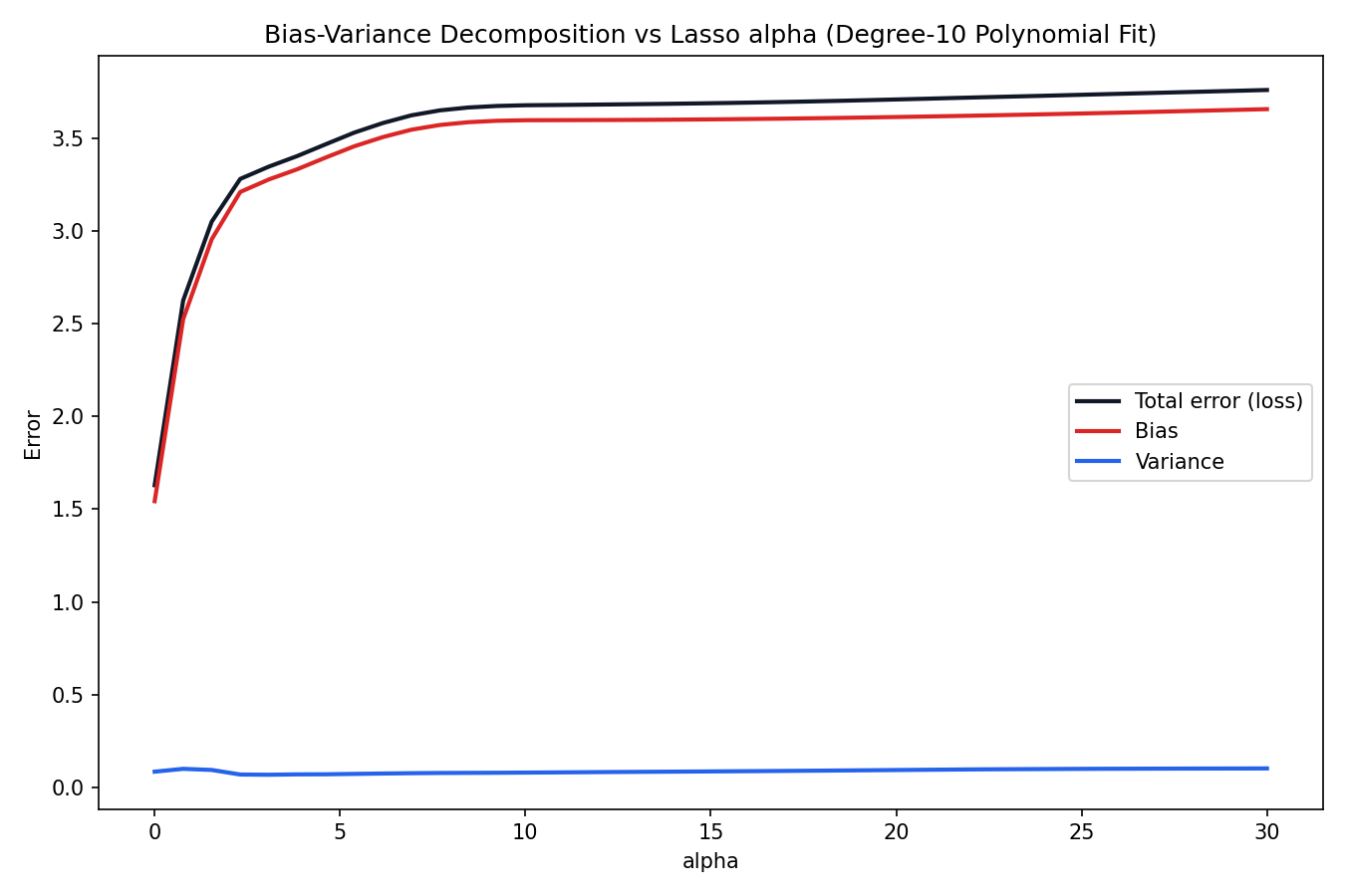

Bias climbs sharply from ≈1.5 to ≈3.6 as alpha rises, exactly as expected: more regularization means a worse fit on the training data. But variance barely moves, drifting between roughly 0.07 and 0.10 across the entire range. Total loss ends up tracking the bias curve almost exactly. This is a real result off this dataset, not a theoretical guarantee, variance in principle should fall as regularization increases, and here it just doesn't fall by much. It's worth treating as an open question rather than a settled one: whether that's specific to this synthetic dataset's degree-10 fit or a more general property of L1 regularization is exactly the kind of thing worth re-running on a different dataset before drawing a firm conclusion.

6. The Loss Function Gets a Kink

The clearest way to see why coefficients hit exactly zero is to look at the loss curve itself, the same single-feature setup from Ch.16's point 4, with the penalty swapped from $\lambda m^2$ to $\lambda |m|$:

def cal_loss(m, alpha):
    return np.sum((y - m * X.ravel() + 2.29) ** 2) + alpha * abs(m)
 
m = np.linspace(-10, 40, 400)
for alpha in [0, 100, 500, 1000, 2500, 3500, 4500, 5500]:
    loss = [cal_loss(mi, alpha) for mi in m]
    # plot m against loss, mark the minimum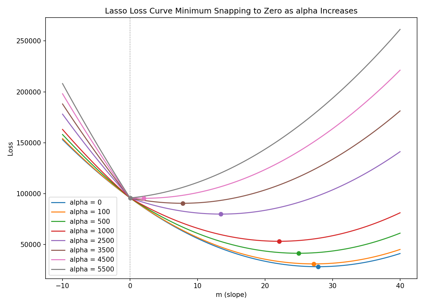

At alpha=0 the minimum sits at m≈27.84, matching unregularized LinearRegression. As alpha climbs through 100, 500, 1000, ..., 5500, the marked minima march steadily left: 27.22, 24.96, 22.08, 13.43, 7.79, 2.03, and finally 0.03, indistinguishable from zero, at alpha=5500.

The reason is visible in the curve shapes themselves. Ridge's $\lambda m^2$ term is smooth everywhere, so its parabola always has a single well-defined bottom that can slide arbitrarily close to the origin without ever touching it exactly, matching the never-quite-zero behavior from Ch.16's point 1. Lasso's $\lambda |m|$ term has a sharp corner, a kink, at $m=0$, since $|m|$ isn't differentiable there. That kink means the loss curve has a genuine V-shaped point at the origin rather than a smooth trough. Once alpha is large enough that the penalty's pull at the kink outweighs whatever the data wants, the minimum snaps directly onto the kink and stays pinned there. No matter how much further alpha increases past that point, the minimum has nowhere left to go, it's already at zero. Working out exactly why a kink forces this snapping behavior, and Ridge's smooth curve doesn't, needs subgradients and is exactly the math the next post covers.

Ridge shrinks every coefficient without ever eliminating one; Lasso eliminates the unimportant ones outright while shrinking the rest. For a dataset with many features that genuinely don't matter, Lasso's automatic feature selection is the practical reason to prefer it over Ridge. The next post works out the math behind why L1's kink produces exact zeros where L2's smooth bowl can't.