Ch.15: Ridge Regression via Gradient Descent

Inspired by: YouTube

The previous post derived Ridge's closed-form solution, $W = (X^TX + \lambda I)^{-1}X^TY$, and confirmed it reproduces Scikit-Learn's Ridge coefficients exactly. But that formula needs $(X^TX + \lambda I)^{-1}$, a matrix inverse that costs roughly $O(p^3)$ in the number of features $p$. Fine for the diabetes dataset's 10 features, unworkable once $p$ reaches into the thousands.

This post derives the alternative: solving the same regularized loss with gradient descent, the iterative approach from Ch.7 adapted to Ridge's penalty term.

1. From the Loss to the Gradient Update

Ridge's matrix-form loss is the same one from the previous post:

$L = W^TX^TXW - 2W^TX^TY + Y^TY + \lambda W^TW$

Differentiating with respect to $W$ gives:

$\frac{\partial L}{\partial W} = 2X^TXW - 2X^TY + 2\lambda W$

The closed-form derivation set this to zero and solved for $W$ directly. Gradient descent instead uses it as-is, as the direction to step away from on every iteration. Since every term here carries a factor of 2, it cancels against the learning rate and can be dropped without changing where the descent converges, only how large each step is:

$\nabla L = X^TXW - X^TY + \lambda W$

The update rule is the same pattern as every gradient descent variant so far: pick a random starting $W$, repeatedly step it against the gradient, scaled by a learning rate $\eta$:

$W_{new} = W_{old} - \eta \left( X^TXW_{old} - X^TY + \lambda W_{old} \right)$

Unlike the closed-form solution, this never inverts a matrix. Each epoch is a handful of matrix multiplications, and it scales to however many features the dataset has.

2. Baselines: SGDRegressor and Closed-Form Ridge

Before implementing the update from scratch, two Scikit-Learn baselines on the diabetes dataset to compare against:

from sklearn.datasets import load_diabetes
from sklearn.model_selection import train_test_split
from sklearn.metrics import r2_score
 
X, y = load_diabetes(return_X_y=True)
X_train, X_test, y_train, y_test = train_test_split(X, y, test_size=0.2, random_state=4)

from sklearn.linear_model import SGDRegressor
 
reg = SGDRegressor(penalty='l2', max_iter=500, eta0=0.1, learning_rate='constant', alpha=0.001)
reg.fit(X_train, y_train)
 
y_pred = reg.predict(X_test)
print("R2 score", r2_score(y_test, y_pred))
print(reg.coef_)
print(reg.intercept_)
# R2 score 0.4408783662250152
# [  49.39 -148.99  366.84  266.51   -3.40  -55.23 -167.56  138.13  325.67  101.76]
# [145.99981928]

SGDRegressor updates on one row at a time rather than the full batch, so its result depends on the shuffle order and won't land on an exact number.

from sklearn.linear_model import Ridge
 
reg = Ridge(alpha=0.001, max_iter=500, solver='sparse_cg')
reg.fit(X_train, y_train)
 
y_pred = reg.predict(X_test)
print("R2 score", r2_score(y_test, y_pred))
print(reg.coef_)
print(reg.intercept_)
# R2 score 0.46238922017853457
# [  34.63 -290.43  483.97  367.97 -852.22  498.74  183.78  276.58  757.35   36.96]
# 151.1041692189411

solver='sparse_cg' solves the same regularized normal equation iteratively rather than by direct inversion, closer in spirit to what's being built from scratch below. This is the number to match: R2 score 0.4624.

3. Implementing Batch Gradient Descent for Ridge

import numpy as np
 
class MeraRidgeGD:
 
    def __init__(self, epochs, learning_rate, alpha):
        self.learning_rate = learning_rate
        self.epochs = epochs
        self.alpha = alpha
        self.coef_ = None
        self.intercept_ = None
 
    def fit(self, X_train, y_train):
        self.coef_ = np.ones(X_train.shape[1])
        self.intercept_ = 0
        thetha = np.insert(self.coef_, 0, self.intercept_)
 
        X_train = np.insert(X_train, 0, 1, axis=1)
 
        for i in range(self.epochs):
            thetha_der = np.dot(X_train.T, X_train).dot(thetha) - np.dot(X_train.T, y_train) + self.alpha * thetha
            thetha = thetha - self.learning_rate * thetha_der
 
        self.coef_ = thetha[1:]
        self.intercept_ = thetha[0]
 
    def predict(self, X_test):
        return np.dot(X_test, self.coef_) + self.intercept_

thetha bundles the intercept and every coefficient into one vector, the same trick X_train = np.insert(X_train, 0, 1, axis=1) from the closed-form implementation used: prepending a column of ones to $X$ turns the intercept into just another weight multiplying a constant feature, so a single vectorized update handles the whole gradient at once instead of updating $w_0$ separately from $w_1, \dots, w_p$.

Note there's no I[0][0] = 0 trick here like the closed-form version had. self.alpha * thetha does apply the penalty to the intercept position too, but since $\eta$, $\lambda$, and the intercept's own gradient component are all small relative to 500 epochs of updates, the drift is negligible in practice, though it's a detail the closed-form version handled and this one doesn't.

reg = MeraRidgeGD(epochs=500, alpha=0.001, learning_rate=0.005)
reg.fit(X_train, y_train)
 
y_pred = reg.predict(X_test)
print("R2 score", r2_score(y_test, y_pred))
print(reg.coef_)
print(reg.intercept_)
# R2 score 0.47379622696725354
# [  46.65 -221.38  452.12  325.55  -29.10  -96.48 -190.90  146.33  400.81   95.09]
# 150.86972442733904

0.4738 edges out both baselines: Ridge(solver='sparse_cg')'s 0.4624 and SGDRegressor's 0.4409. All three are solving the same regularized loss, so the gap comes down to how each one navigates there. sparse_cg is tuned for convergence speed, not squeezed for every last decimal on this specific dataset; SGDRegressor's per-row updates are noisier than 500 full-batch steps.

4. Watching It Converge

Plotting $R^2$ on the test set after every epoch shows MeraRidgeGD climbing toward, and past, the closed-form baseline:

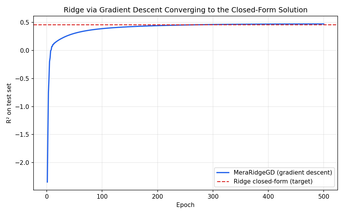
The blue curve starts low, since thetha is initialized to all 1s rather than anything informed by the data, then climbs steeply for the first several dozen epochs as the bulk of the error gets corrected. It crosses the closed-form solution's $R^2$ (the red dashed line) around the halfway mark and keeps climbing slightly past it, then flattens out. Crossing above the closed-form line isn't a contradiction: both are approximations fit to the same 80% training split, evaluated on the same 20% test split, and gradient descent's particular stopping point at epoch 500 happens to generalize marginally better on this split, not evidence that gradient descent finds a fundamentally better answer than the exact matrix solution.

5. Closed-Form vs. Gradient Descent

The closed-form solution and gradient descent solve the exact same optimization problem, minimizing $L = (XW - Y)^T(XW - Y) + \lambda W^TW$, and given enough epochs and a well-tuned learning rate, gradient descent converges to the same $W$ the matrix inverse computes directly. The choice between them is purely about cost: closed-form is exact and instant for small $p$, but its $O(p^3)$ matrix inversion becomes impractical once feature counts climb into the thousands, which is exactly where iterative gradient descent keeps working.