
Ch.71: Hyperparameter Tuning with Optuna and Bayesian Optimization
Inspired by: YouTube
1. The Problem: Picking Hyperparameters
Take the familiar placement problem: for each student we have a CGPA and an IQ, and we want to predict whether they'll get placed. We've decided to use a random forest, and we want the accuracy to be as high as possible.
A random forest has hyperparameters, settings we choose before training rather than values the model learns. Focus on two of them:
max_depth: how deep each decision tree is allowed to grow.n_estimators: how many decision trees the forest contains.
Different values give different accuracies, and there is no way to know the best pair in advance. So we search: pick some candidate values, train the model on each combination, and keep whichever scores best. This is hyperparameter tuning.
The first step is always to define a search space, the values you're willing to try, using intuition and domain knowledge. Say we try max_depth from 1 to 5, and n_estimators from 50 to 250 in steps of 50 (50, 100, 150, 200, 250). That's 5 values for each, and every pairing of them is a candidate, so the search space is a 5 by 5 grid of 25 combinations.
The question this post answers: which of those 25 cells should we actually spend time training on?
2. Grid Search: Try Everything
The most direct answer is to try them all. Grid search (scikit-learn's GridSearchCV, covered in Ch.52) walks the grid cell by cell. It trains with max_depth=1, n_estimators=50 and records the accuracy, say 71%. Then max_depth=1, n_estimators=100: 69%. Then max_depth=1, n_estimators=150: 74%. And so on through all 25 cells, after which it returns the combination with the highest score.
Because it checks everything, it's guaranteed to find the best cell in the grid. The problem is what that guarantee costs.
The number of combinations multiplies. Every hyperparameter's list of values multiplies the size of the grid:
| Search space | Combinations |
|---|---|
max_depth 1 to 5, 5 values of n_estimators | 5 × 5 = 25 |
Add one more value of n_estimators (6 values) | 5 × 6 = 30 |
Widen max_depth to 1 to 20 | 20 × 5 = 100 |
Back to 5 × 5, plus min_samples_split with 3 values | 5 × 5 × 3 = 75 |
| Plus a fourth hyperparameter with 4 values | 5 × 5 × 3 × 4 = 300 |
Adding one value to one list adds a whole row of the grid. Adding a whole new hyperparameter multiplies everything you had by its number of values. A realistic search over five or six hyperparameters runs into thousands of combinations.
And every combination is a full training run. The total cost is
On a small tabular dataset, one fit takes a fraction of a second, so even 300 fits are tolerable. Deep learning is where this breaks: a neural network on a large dataset can take an hour or more to train once. At an hour per fit, the modest 25-cell grid is already a full day of compute, and the 300-cell grid is nearly two weeks. Grid search gives the best answer in the grid, but in many real settings you can't afford to ask it the question.
3. Random Search: Try a Few, at Random
Random search (RandomizedSearchCV) attacks the cost directly. You give it a budget, say 5 trials, and it picks 5 random cells from the grid, trains on those, and returns the best of the 5. Doubling the search space no longer doubles the cost; the budget stays whatever you set.
What it gives up is the guarantee. The best combination might sit in a cell random search never landed on. Nothing pulls it toward that cell, so it simply returns the best of whatever it happened to try, and you're left with a worse configuration than one that was available.
4. What Both Have in Common: No Memory
Grid search and random search look like opposites, one exhaustive and one sparse, but they share a deeper flaw. Neither one uses the results of earlier trials to decide what to try next.
When grid search finishes its 10th combination, it moves to the 11th because that's the next cell in the grid, not because anything about the first 10 results suggested it. When random search picks its 11th combination, it's a fresh random draw, identical to what it would pick if the first 10 had never happened. If the first ten trials all showed that shallow trees score badly, both methods will happily keep spending trials on shallow trees.
That's the sense in which they're called "dumb" searches. It isn't that they're brute force (random search isn't), it's that each trial is chosen blind. Information is being thrown away after every single run.
5. Bayesian Search: Learn From Every Trial
Optuna's main strength is that it searches a different way, using Bayesian search (also called Bayesian optimization), an approach rooted in probability. The full mathematics is a topic of its own, but the intuition is straightforward.
Step 1: accuracy is a function of the hyperparameters. If changing max_depth from 5 to 25 changes the accuracy, and changing n_estimators from 10 to 100 changes it too, then there must be some relationship between them:
Plot it with max_depth on one axis, n_estimators on another and accuracy on the vertical axis, and is a surface. Finding the best hyperparameters means finding the highest point on that surface.
This is a real function, it just has no formula. "Function" in mathematics means a mapping: every input gets exactly one output. Give the input max_depth=15, n_estimators=100 and, with the random seed fixed, it returns the same accuracy every time, so it genuinely is a function. What it doesn't have is an equation you can write down like . The only way to learn its value at a point is to compute it: train a model with those hyperparameters and measure the accuracy. A function you can evaluate but can't look inside is called a black-box function.
Step 2: each trial reveals one point on the surface. Train with max_depth=5, n_estimators=100, get 75%, and you now know one point on . Train with max_depth=10, n_estimators=150, get 69%, and you know a second.
To see this concretely, drop to one dimension: fix n_estimators at 100 and look only at how accuracy changes with max_depth. Below, the left panel shows what a search knows after three trials, at max_depth 5, 10 and 15, on the real dataset used later in this post. The right panel shows the full curve those three points come from, computed by training at every depth from 1 to 20.
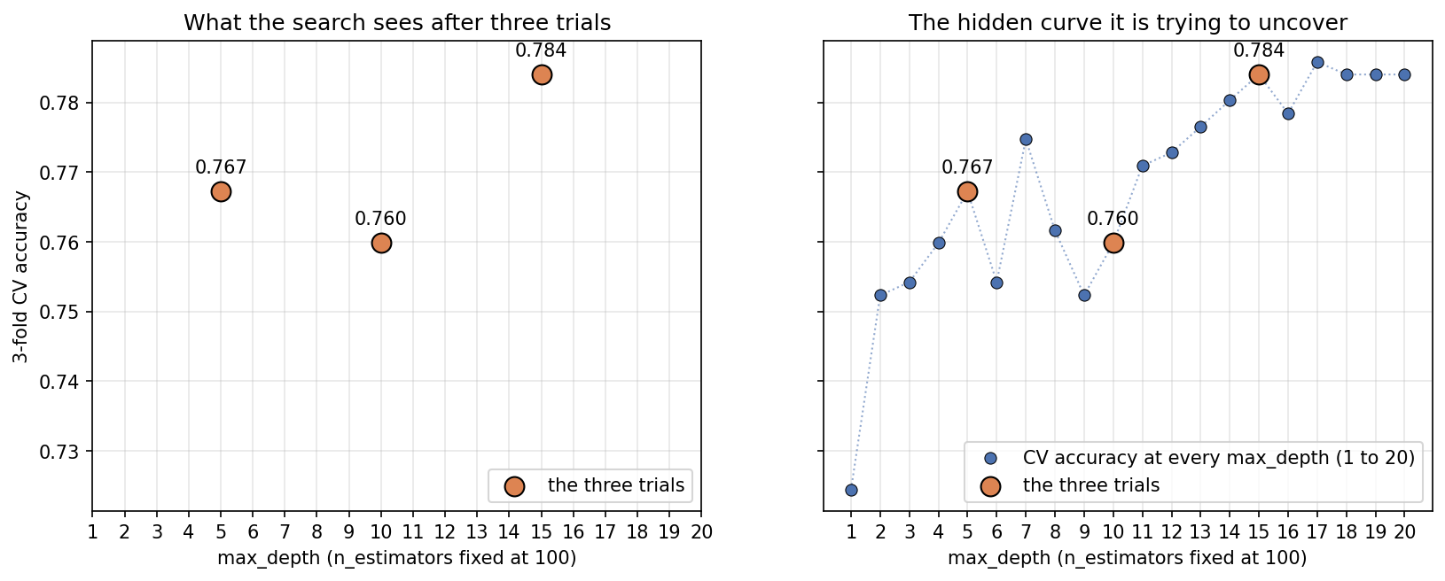
From the left panel alone, three points already suggest something: deeper looks better, and the region around 15 is worth exploring further. Bayesian search turns that suggestion into a decision. After each trial, it updates its estimate of what the whole surface probably looks like, then picks the next trial where that estimate says a high score is likely. The new result refines the estimate, which picks the next trial, and so on.
Step 3: concentrate on promising regions. Over many trials, the search gradually uncovers the shape of the surface and spends more and more of its budget near the peaks, while largely abandoning regions that have already scored badly. It uses far fewer trials than grid search, and unlike random search, every trial is informed by all the ones before it.
That's the core difference:
| Uses past trials to choose the next one? | Cost | |
|---|---|---|
| Grid search | No | Every combination |
| Random search | No | Fixed budget |
| Bayesian search | Yes | Fixed budget, spent where it's most promising |
6. Why Not Just Use Gradient Descent?
If the best hyperparameters are the highest point on a surface, an obvious question follows. Gradient descent already finds the lowest point of a loss surface; flip the sign and it finds the highest. Why invent a different search at all?
Because gradient descent depends on things this surface doesn't have. It works by computing the slope (the gradient) at the current point and taking a small step downhill, thousands of times. Each of those requirements fails here.
1. There is no formula to differentiate. When gradient descent trains linear or logistic regression, the loss is an explicit formula in the weights, so the gradient is an explicit formula too: compute it, step, repeat. Here the "formula" is "train a random forest with these settings and score it." There is no expression in max_depth to differentiate. You could try to estimate the slope by training at two nearby points and comparing, but that leads straight into the next two problems.
2. Most hyperparameters aren't continuous. Gradient descent moves by small, continuous steps: from 4.00 to 3.97 to 3.95. But max_depth can be 7 or 8, never 7.5. n_estimators is a count of trees. Later in this post, the kernel of an SVM ('linear', 'rbf', ...) and even the choice of algorithm itself become hyperparameters, and there is nothing "between" 'SVM' and 'RandomForest' to take a slope over. A gradient needs a direction to move in continuously, and these values only exist at separate points.
3. Even where you can probe nearby values, the surface is flat steps and sudden jumps. Here is the real cross-validated accuracy at every single n_estimators value from 50 to 200, with max_depth fixed at 15:
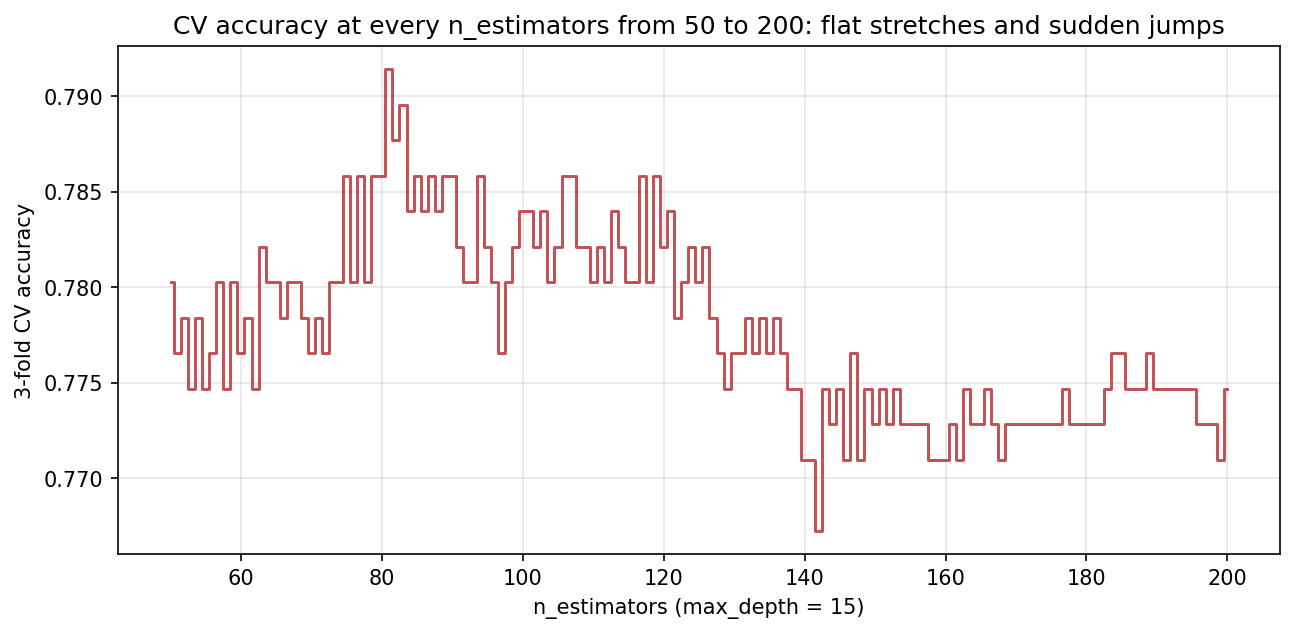
Across those 151 settings, the accuracy takes only 13 distinct values, and in 40 of the 150 steps from one value to the next it doesn't change at all (100 trees and 101 trees both give 0.7840). This isn't a quirk of this dataset; it comes from how accuracy is measured. Accuracy counts correct predictions. Each of the three folds holds 179 training rows, so the averaged accuracy can only move in steps of : one more or one fewer correct prediction. Every jump in the chart is a multiple of that. On a flat stretch the slope is exactly zero, so gradient descent has no direction to move in, and at a jump the slope isn't defined at all. (This is the same reason models are trained on a smooth loss like log loss rather than on accuracy directly.)
4. Every step would be a full training run. Gradient descent's strength is taking many cheap steps. Here each evaluation of means training a model, three times over with 3-fold cross-validation. A thousand gradient steps would cost three thousand trainings, and that's before estimating any slopes. Bayesian search is designed for exactly the opposite situation: evaluations are expensive, so make each one count and stop after tens of trials, not thousands.
5. The surface is bumpy. The max_depth curve in the previous section dips at 6, 8 and 9 between higher values, and the n_estimators chart has spikes and valleys everywhere. Even with a usable gradient, a local method could get stuck on a minor bump. This matters, but it's the least fundamental of the five: Bayesian search can also miss the true peak. The real reasons are the first four. You can only probe the surface one expensive training run at a time, many inputs are discrete, and accuracy is flat almost everywhere.
7. Optuna's Five Key Terms
Five terms appear in every piece of Optuna code.
- Study: the whole tuning task. "Find the best
max_depthandn_estimatorsfor a random forest on this dataset" is one study. Formally, a study is an optimization session made up of many trials. - Trial: one single run. Pick one combination, train the model, record the score. A study with 50 trials trains 50 times, and the best of those trials gives the best hyperparameters.
- Trial parameters: the specific hyperparameter values used in one trial, for example
max_depth=2, n_estimators=100. - Objective function: the black box from section 5, written as code. It takes hyperparameter values in and returns the score out. You write it yourself: it builds the model, trains it, and returns the metric.
- Sampler: the component that decides which hyperparameters the next trial should use, based on all the trials so far. This is where the Bayesian intelligence lives. Optuna's default sampler is TPE, the Tree-structured Parzen Estimator. You don't need its internal mathematics to use it; the TPE paper covers it in detail for anyone curious, as does the Optuna paper for the framework as a whole.
8. Optuna in Code
The code below follows the source notebook. It uses the Pima Indians Diabetes dataset: 768 patients, 8 medical measurements each, and whether they have diabetes (500 don't, 268 do). It's a classification dataset where good results don't come easily, which makes it a useful testbed for tuning.
!pip install optunaimport optuna
import numpy as np
import pandas as pd
from sklearn.model_selection import train_test_split
from sklearn.preprocessing import StandardScaler
url = "https://raw.githubusercontent.com/jbrownlee/Datasets/master/pima-indians-diabetes.data.csv"
columns = ['Pregnancies', 'Glucose', 'BloodPressure', 'SkinThickness', 'Insulin', 'BMI',
'DiabetesPedigreeFunction', 'Age', 'Outcome']
df = pd.read_csv(url, names=columns)The dataset has a known problem: missing values are recorded as 0. A blood pressure or BMI of 0 isn't possible, yet 35 rows have a blood pressure of 0, and 374 of the 768 rows have an insulin of 0. So the zeros in those columns are replaced with NaN and then filled with the column mean.
cols_with_missing_vals = ['Glucose', 'BloodPressure', 'SkinThickness', 'Insulin', 'BMI']
df[cols_with_missing_vals] = df[cols_with_missing_vals].replace(0, np.nan)

X = df.drop('Outcome', axis=1)
y = df['Outcome']

X_train, X_test, y_train, y_test = train_test_split(X, y, test_size=0.3, random_state=42)

# fill missing values with means computed from the training rows only
train_means = X_train.mean()
X_train = X_train.fillna(train_means)
X_test = X_test.fillna(train_means)

scaler = StandardScaler()
X_train = scaler.fit_transform(X_train)
X_test = scaler.transform(X_test)

print(f'Training set shape: {X_train.shape}')
print(f'Test set shape: {X_test.shape}')
Training set shape: (537, 8)
Test set shape: (231, 8)
One deliberate difference from the source notebook: it fills the missing values with means from the whole dataset before splitting, which lets a little information from the test rows leak into training. Here the means come from the training rows only. Scaling isn't really needed for a random forest, since trees split on thresholds and don't care about feature scale, but it does no harm.
The objective function
This is where all the real work happens, and it does two things: defines the search space, and trains a model with values drawn from it.
from sklearn.ensemble import RandomForestClassifier
from sklearn.model_selection import cross_val_score

def objective(trial):
    # Search space: Optuna suggests a value for each hyperparameter
    n_estimators = trial.suggest_int('n_estimators', 50, 200)
    max_depth = trial.suggest_int('max_depth', 3, 20)

    model = RandomForestClassifier(
        n_estimators=n_estimators,
        max_depth=max_depth,
        random_state=42
    )

    # 3-fold cross-validation accuracy, averaged
    score = cross_val_score(model, X_train, y_train, cv=3, scoring='accuracy').mean()

    return score
trial.suggest_int('n_estimators', 50, 200) says: "this hyperparameter is an integer between 50 and 200; give me a value to try." Unlike the grid in section 1, which only allowed multiples of 50, every integer in the range is fair game: 51, 69 and 122 are all possible.
The trial object is the link to the sampler. Each time objective is called, Optuna passes in a fresh trial, and when the code calls suggest_int, the sampler chooses the value based on every trial so far. The rest is ordinary training: build the model, run 3-fold cross-validation, return the mean accuracy. That returned number is evaluated at one point.
Creating and running the study
Two lines run the entire search:
study = optuna.create_study(direction='maximize', sampler=optuna.samplers.TPESampler(seed=42))
study.optimize(objective, n_trials=50)
create_study sets up the study and needs two things:
direction: whether a higher or lower return value is better. Accuracy should be as high as possible, so this is'maximize', and the same goes for any score where higher is better, like . If the objective returned a loss instead (log loss, mean squared error), it would have to be'minimize'.sampler: which strategy picks the next trial. TPE is the default even if you leave this out; it's written explicitly here for clarity, with a fixedseedso the run is reproducible.
Getting direction wrong doesn't cause an error, and that's exactly what makes it dangerous. Optuna has no idea what your number means; it only knows which way you said is better. Return a log loss but leave direction='maximize', and Optuna will diligently steer every trial toward the settings that make the model's predictions as bad as possible, then report the worst configuration it found as the "best" one, with no warning. Whenever you change what the objective returns, check the direction.
optimize then runs the loop 50 times: the sampler proposes values, objective trains and returns a score, the sampler updates its picture of the surface and proposes the next values.
Trial 0 finished with value: 0.7896 and parameters: {'n_estimators': 106, 'max_depth': 20}.
Trial 1 finished with value: 0.7728 and parameters: {'n_estimators': 160, 'max_depth': 13}.
Trial 2 finished with value: 0.7728 and parameters: {'n_estimators': 73, 'max_depth': 5}.
Trial 3 finished with value: 0.7765 and parameters: {'n_estimators': 58, 'max_depth': 18}.
...
After 50 trials, the study holds the best result:
print(f'Best trial accuracy: {study.best_trial.value}')
print(f'Best hyperparameters: {study.best_trial.params}')
Best trial accuracy: 0.7895716945996275
Best hyperparameters: {'n_estimators': 106, 'max_depth': 20}
That 79% is cross-validated accuracy on the training data. To check it on unseen data, train a fresh model with those values and score it on the test set:
from sklearn.metrics import accuracy_score

best_model = RandomForestClassifier(**study.best_trial.params, random_state=42)
best_model.fit(X_train, y_train)
y_pred = best_model.predict(X_test)
print(f'Test Accuracy with best hyperparameters: {accuracy_score(y_test, y_pred):.2f}')
Test Accuracy with best hyperparameters: 0.74
A genuine quirk in this run: the best trial is trial 0, the very first one, and none of the following 49 trials beat it. That's not TPE failing. TPE needs some data before it can model anything, so its first 10 trials are random by default. Here, the first random draw happened to land on a strong spot (deep trees, around 100 of them), and the rest of the search never found anything higher. Section 10 shows this directly.
9. Grid and Random Search Inside Optuna
Optuna isn't limited to Bayesian search. It ships several samplers, and swapping the sampler makes the same objective run as random search or grid search, with no scikit-learn search classes needed.
Random search:
study = optuna.create_study(direction='maximize', sampler=optuna.samplers.RandomSampler(seed=42))
study.optimize(objective, n_trials=50)
Grid search needs the grid written out explicitly, since it tries every cell. Four values each gives 4 × 4 = 16 trials:
search_space = {
    'n_estimators': [50, 100, 150, 200],
    'max_depth': [5, 10, 15, 20]
}

study = optuna.create_study(direction='maximize', sampler=optuna.samplers.GridSampler(search_space))
study.optimize(objective)
The results from all three on this dataset:
| Sampler | Trials | Best CV accuracy | Best hyperparameters | Test accuracy |
|---|---|---|---|---|
| TPE (Bayesian) | 50 | 0.7896 | n_estimators=106, max_depth=20 | 0.74 |
| Random | 50 | 0.7896 | n_estimators=106, max_depth=20 | 0.74 |
| Grid | 16 | 0.7840 | n_estimators=100, max_depth=20 | 0.74 |
TPE and random search returned the identical answer, and the reason is the quirk from the end of section 8. TPE's first 10 trials are random, and with the same seed they're exactly the same 10 random trials random search makes. Both started with the same lucky trial 0, and neither ever beat it.
The best scores alone hide the real difference, which is where each sampler spent its trials:
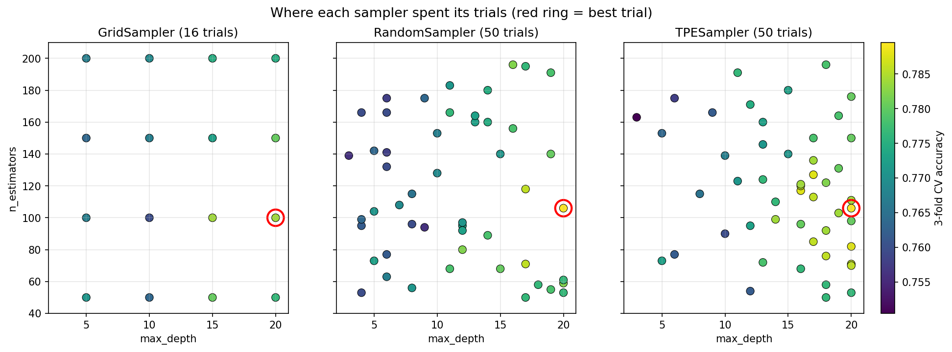
Grid search covers the space evenly and blindly. Random search scatters its trials all over, spending just as many on shallow, poorly scoring trees as on deep ones: exactly half its trials have max_depth of 12 or more. TPE starts out the same way, then piles its trials into the bright region on the right: 78% of its trials have max_depth of 12 or more. That's the learning from section 5, made visible. It found that deep trees score better and stopped wasting trials on shallow ones.
So why didn't it end up with a better score? Because on this dataset, the high region is a broad plateau of roughly 0.78 to 0.79 with no single sharp peak to find. The gaps between the samplers' best results are one or two correct predictions out of 537, the size of the steps from section 6. On a small dataset like this, careful searching and lucky searching land in the same place. The difference matters on larger problems with sharper peaks, and especially where each trial is expensive enough that you can't afford to waste half your budget on regions already known to be bad.
One more honest observation. While generating the step chart in section 6, the single highest accuracy appeared at n_estimators=81, max_depth=15, scoring 0.7914, higher than anything any of the three samplers found. It's a narrow spike: 80 trees score 0.7858 and 82 score 0.7877. That's a good reminder not to over-trust a "best" value that beats its neighbors by a hair. A spike that thin is mostly noise from which rows happened to fall into which fold, and it won't reliably carry over to new data.
10. Visualizing a Study
Once a study finishes, Optuna can plot what happened, which is one of its most useful features. Each plot below comes from the 50-trial TPE study above.
from optuna.visualization import (plot_optimization_history, plot_parallel_coordinate,
                                  plot_slice, plot_contour, plot_param_importances)
Optimization history plots every trial's score against its trial number, with a line tracking the best score so far.
plot_optimization_history(study).show()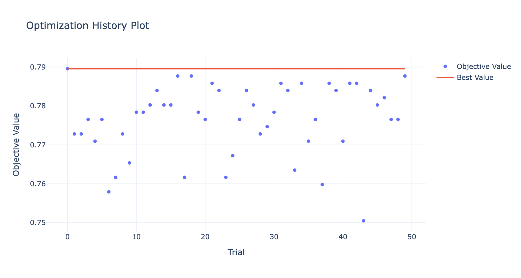
Normally the best-value line climbs in steps as the search finds better configurations, then flattens out once it stops improving, which tells you roughly how many trials a problem needs. Here it's flat from the start because trial 0 was the best. The dots still show the search improving: the first ten random trials are scattered widely, and after trial 10, when TPE takes over, most trials sit between 0.77 and 0.79. The typical trial got better even though the best didn't. It still occasionally tries something far away, like trial 43 at max_depth=3, the lowest score of the study: a learning sampler keeps exploring a little, so it can notice if its picture of the surface is wrong.
Parallel coordinate plot draws each trial as a line crossing a vertical axis for each quantity: the score, then each hyperparameter. Darker lines are higher scores.
plot_parallel_coordinate(study).show()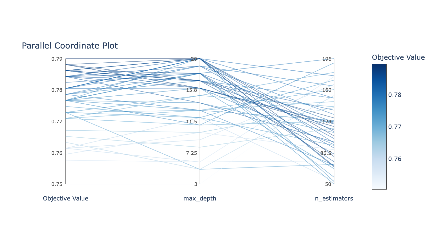
Where lines bunch together on an axis, that's where the search concentrated. On max_depth, most lines, and nearly all the dark ones, pass between roughly 16 and 20: that's the region TPE judged promising. On n_estimators they spread much more widely, a hint that this hyperparameter matters less.
Slice plot shows each hyperparameter against the score separately, one panel each, with dots colored by trial number.
plot_slice(study).show()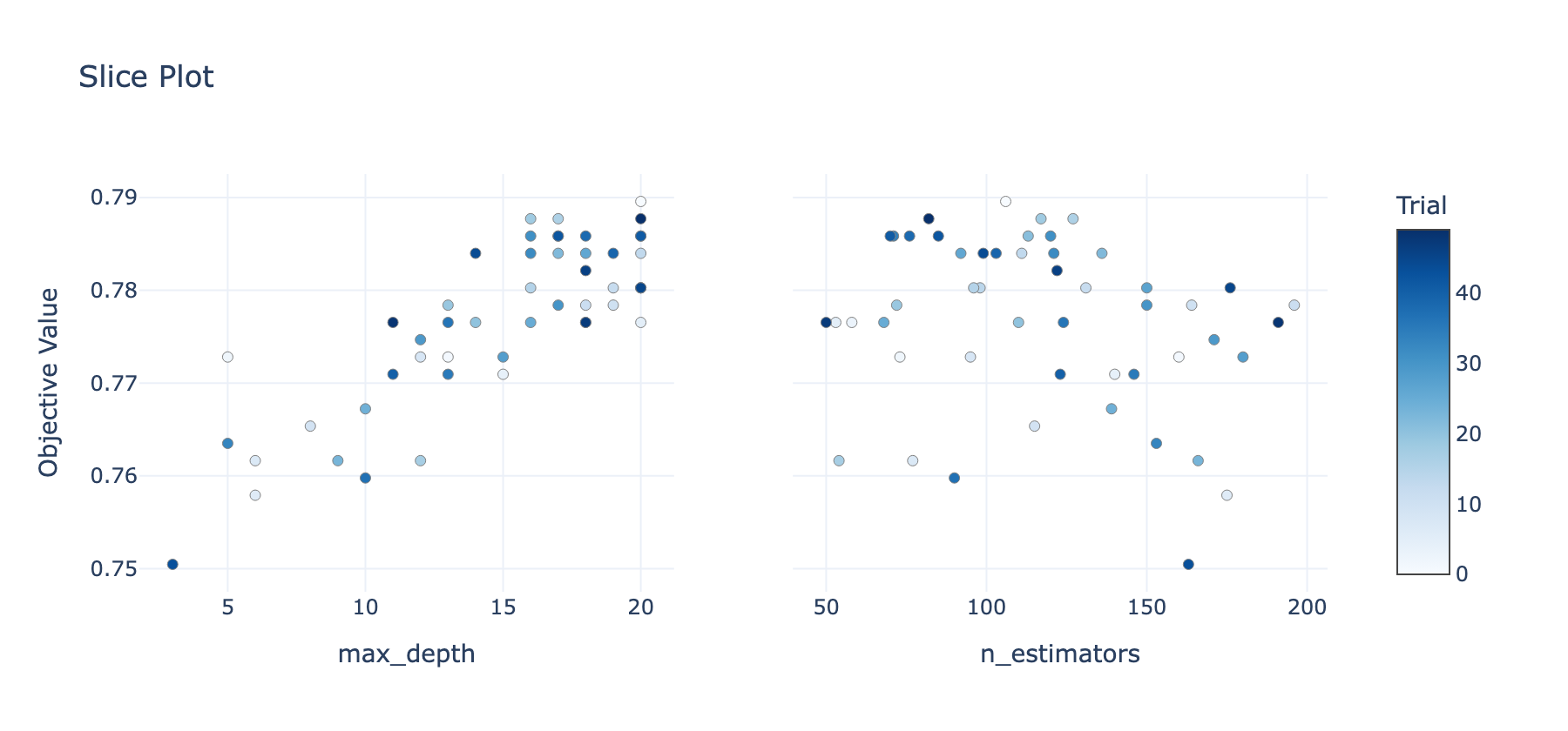
The left panel makes the max_depth relationship obvious: deeper trees score higher, and most trials (especially later, darker ones) sit at the deep end. The right panel shows no clear trend for n_estimators at all.
Contour plot shows the estimated surface from section 5 from above: max_depth across, n_estimators up, and color for the score, darker meaning higher. The dots are the trials.
plot_contour(study).show()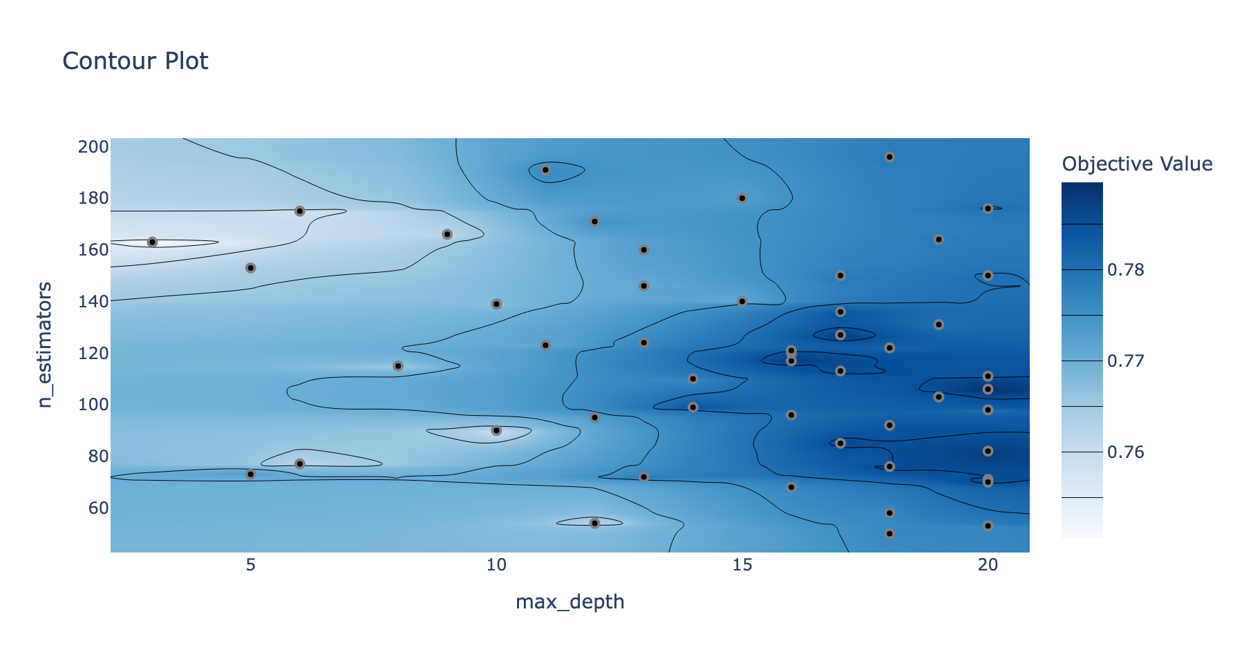
This is the most direct picture of what Bayesian search does. The pale left side, shallow trees, scored poorly, and TPE rarely went back there. The dark region on the right, deep trees with roughly 70 to 130 estimators, is the hot spot, and that's where the dots pile up. The search found the promising region and spent its energy there.
Hyperparameter importances estimate how much each hyperparameter affected the score across the study.
plot_param_importances(study).show()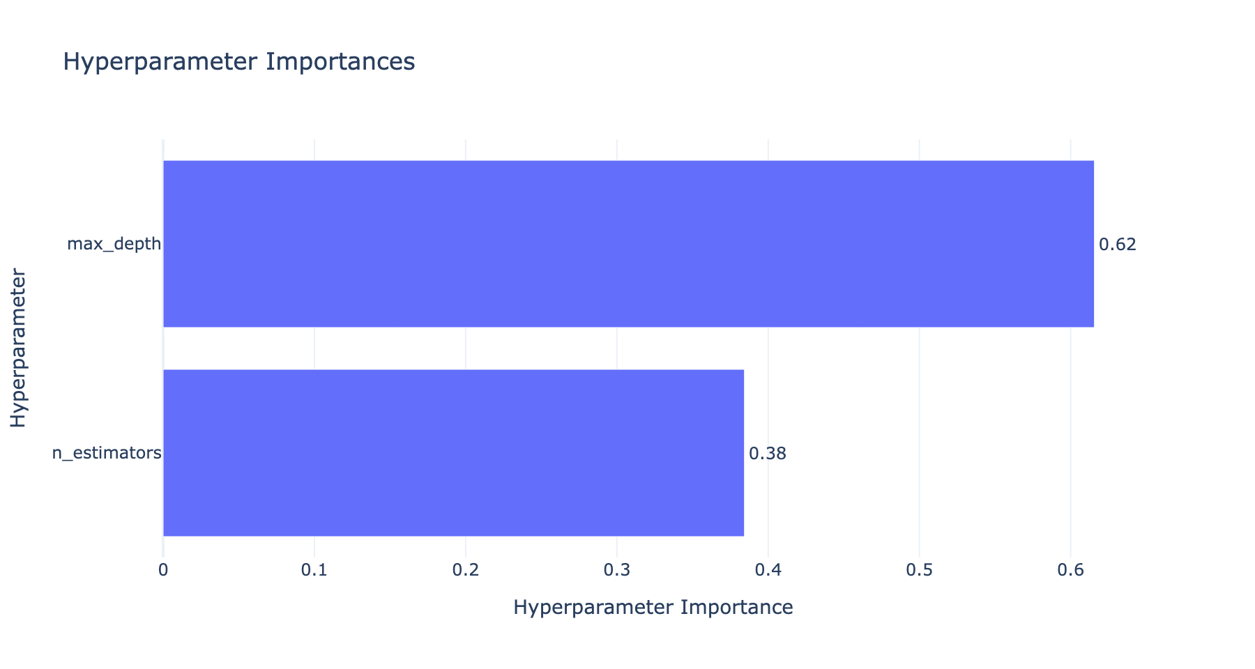
max_depth accounts for about 62% and n_estimators about 38%, matching what the slice and parallel coordinate plots suggested. These importances are estimated from this one study's trials, so the exact split shifts from run to run, but the ranking is a practical guide: if you tune this model again, spend your search effort on max_depth.
11. Define-by-Run: Tuning the Choice of Algorithm Too
So far we decided up front that a random forest was the right model. But in practice you rarely know that in advance. Logistic regression, SVM, random forest and gradient boosting might each win on a given dataset, and the usual approach is to tune each one separately and compare. Four algorithms means four complete tuning runs.
Optuna can do it all in one study, by treating the choice of algorithm as a hyperparameter itself. And because the search space is defined inside the objective function, as ordinary Python code that runs each trial, the rest of the search space can depend on that choice. If the algorithm is SVM, tune SVM's hyperparameters; if it's random forest, tune the forest's. Optuna calls this define-by-run: the search space is defined as the code runs, so it can branch.
from sklearn.ensemble import RandomForestClassifier, GradientBoostingClassifier
from sklearn.svm import SVC

def objective(trial):
    # The algorithm itself is a hyperparameter
    classifier_name = trial.suggest_categorical('classifier', ['SVM', 'RandomForest', 'GradientBoosting'])

    if classifier_name == 'SVM':
        c = trial.suggest_float('C', 0.1, 100, log=True)
        kernel = trial.suggest_categorical('kernel', ['linear', 'rbf', 'poly', 'sigmoid'])
        gamma = trial.suggest_categorical('gamma', ['scale', 'auto'])
        model = SVC(C=c, kernel=kernel, gamma=gamma, random_state=42)

    elif classifier_name == 'RandomForest':
        n_estimators = trial.suggest_int('n_estimators', 50, 300)
        max_depth = trial.suggest_int('max_depth', 3, 20)
        min_samples_split = trial.suggest_int('min_samples_split', 2, 10)
        min_samples_leaf = trial.suggest_int('min_samples_leaf', 1, 10)
        bootstrap = trial.suggest_categorical('bootstrap', [True, False])
        model = RandomForestClassifier(
            n_estimators=n_estimators, max_depth=max_depth,
            min_samples_split=min_samples_split, min_samples_leaf=min_samples_leaf,
            bootstrap=bootstrap, random_state=42
        )

    elif classifier_name == 'GradientBoosting':
        n_estimators = trial.suggest_int('n_estimators', 50, 300)
        learning_rate = trial.suggest_float('learning_rate', 0.01, 0.3, log=True)
        max_depth = trial.suggest_int('max_depth', 3, 20)
        min_samples_split = trial.suggest_int('min_samples_split', 2, 10)
        min_samples_leaf = trial.suggest_int('min_samples_leaf', 1, 10)
        model = GradientBoostingClassifier(
            n_estimators=n_estimators, learning_rate=learning_rate, max_depth=max_depth,
            min_samples_split=min_samples_split, min_samples_leaf=min_samples_leaf, random_state=42
        )

    score = cross_val_score(model, X_train, y_train, cv=3, scoring='accuracy').mean()
    return score
Every value here, including the classifier, the SVM's C and kernel, and the forest's min_samples_leaf, is chosen by the TPE sampler. Two new suggestion types appear: suggest_categorical picks from a list of options, and suggest_float(..., log=True) samples on a logarithmic scale, so values between 0.1 and 1 get as much attention as values between 10 and 100. After the branches, whichever model was built is trained and scored the same way.
Running it is the same two lines as before, with more trials since the search space is much larger:
study = optuna.create_study(direction='maximize', sampler=optuna.samplers.TPESampler(seed=42))
study.optimize(objective, n_trials=100)

print("Best trial parameters:", study.best_trial.params)
print("Best trial accuracy:", study.best_trial.value)
Best trial parameters: {'classifier': 'RandomForest', 'n_estimators': 120, 'max_depth': 12, 'min_samples_split': 3, 'min_samples_leaf': 9, 'bootstrap': False}
Best trial accuracy: 0.7877094972067039
study.trials_dataframe() returns every trial as a pandas DataFrame, with its score, start and finish times, duration, and the value of every hyperparameter. That makes it easy to ask how the 100 trials were split between the algorithms, and how each one scored on average:
study.trials_dataframe()['params_classifier'].value_counts()
study.trials_dataframe().groupby('params_classifier')['value'].mean()| Algorithm | Trials | Mean CV accuracy | Best CV accuracy |
|---|---|---|---|
| SVM | 65 | 0.7728 | 0.7877 |
| RandomForest | 25 | 0.7712 | 0.7877 |
| GradientBoosting | 10 | 0.7425 | 0.7672 |
This table shows both the strength and the risk of a sampler that learns.
The strength: gradient boosting scored clearly worse (a 0.7425 average), so the sampler gave it only 10 of the 100 trials. It also saw that SVM was scoring well on average, and in the last 30 trials it chose SVM 24 times, random forest 4 times, and gradient boosting twice. One study tuned three algorithms, and the budget flowed to where the results were.
The risk: it concentrates on whatever looked best early, and early impressions are based on few trials. Notice that SVM received 65 trials, but the best trial of the whole study is a random forest, and SVM's best only ties it. The SVM average (0.7728) beats the random forest average (0.7712) by less than one correct prediction out of 537, a difference well within noise. If a model's good settings occupy a narrow region of its search space, its first few random trials can easily miss them, it looks worse than it is, and it may never get enough trials to show what it can do. The sampler still gives every option some trials, which is what kept random forest in the running here, but this is why it's worth looking at the per-algorithm breakdown rather than accepting the single best result blindly.
12. Beyond This Post
A few more features make Optuna a strong default for hyperparameter tuning:
- Distributed optimization: trials can run in parallel on multiple machines, sharing one study, for a much faster search.
- Integrations: Optuna works well with scikit-learn, Keras, PyTorch and MLflow, so the same workflow carries from classical machine learning into deep learning.
The workflow itself stays small however big the problem gets: write an objective function that builds, trains and scores a model with values from trial.suggest_*, create a study with the right direction, and call optimize. Everything clever happens in the sampler, which turns every finished trial into a better guess about where to look next.