
Ch.70: Imbalanced Data, Undersampling, Oversampling, SMOTE and Beyond
Inspired by: YouTube
1. What Imbalanced Data Is
Take a classification problem: a college has records of its final-year students, each with a CGPA, an IQ, and whether the student got placed. The goal is a model that, given a new student's CGPA and IQ, predicts whether they'll be placed.
Now suppose the college is a very good one, where nearly everyone gets placed. Out of 1,000 students, 900 were placed and 100 weren't. That's imbalanced data: the two classes the model must tell apart appear in very different proportions. The larger one (placed) is the majority class; the smaller one (not placed) is the minority class.
It isn't limited to two classes. If 10 students at the same college skipped placements entirely, that's a three-class problem (placed, not placed, didn't participate), and it's still imbalanced: one class dominates and the other two are small.
2. Why It's a Problem
So the classes are uneven. Why should that matter? Two separate reasons.
Problem 1: the model becomes biased toward the majority class. A model learns patterns from the examples it sees. With 900 majority examples and 100 minority ones, most of what it sees, and therefore most of what it learns from, is the majority class. Getting the majority right reduces the training error far more than getting the minority right, so that's what the model optimizes for. The result is a model that's good on the majority class and poor on the minority class.
Problem 2: accuracy stops being a reliable metric. Imagine the dumbest possible model, one that ignores its input and always answers "placed." On the 900/100 data, it's right 900 times out of 1,000: 90% accuracy, without having learned anything. It can't identify a single unplaced student, yet the headline number looks respectable.
Both problems are easy to see on real data. The dataset used throughout this post comes from the source notebook: 400 two-dimensional points generated as two overlapping blobs, 25 in one class and 375 in the other.
import numpy as np
import matplotlib.pyplot as plt
from sklearn.datasets import make_blobs
from sklearn.model_selection import train_test_split

X, y = make_blobs(n_samples=[25, 375],
                  centers=[(0, 0), (2, 2)],
                  cluster_std=[1.5, 1.5],
                  random_state=0)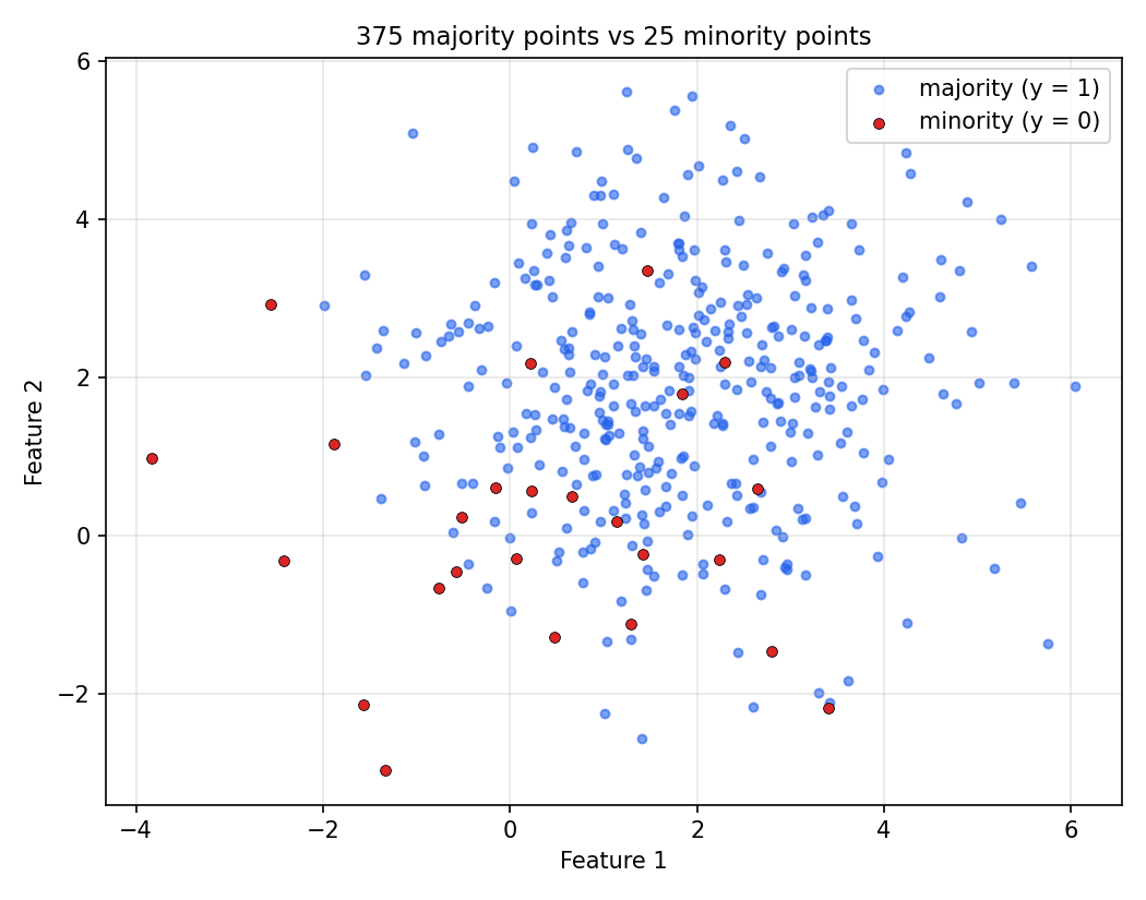
One labeling detail to keep straight: make_blobs gives the first group label 0, so here the minority class is y = 0 and the majority is y = 1. That matters later, when terms like "false positive" come up.
Training a plain logistic regression on this:
from sklearn.linear_model import LogisticRegression
from sklearn.metrics import classification_report, roc_auc_score

X_train, X_test, y_train, y_test = train_test_split(X, y, test_size=0.3, random_state=42)

classifier = LogisticRegression()
classifier.fit(X_train, y_train)

y_pred = classifier.predict(X_test)
y_proba = classifier.predict_proba(X_test)[:, 1]
print(classification_report(y_test, y_pred))
print("ROC AUC Score:", roc_auc_score(y_test, y_proba))
precision recall f1-score support
0 1.00 0.29 0.44 7
1 0.96 1.00 0.98 113
accuracy 0.96 120
macro avg 0.98 0.64 0.71 120
weighted avg 0.96 0.96 0.95 120
ROC AUC Score: 0.9557522123893806
96% accuracy. In most projects that number would be cause for celebration. But look at the row for class 0, the minority: its recall is 0.29. Of the 7 minority points in the test set, the model correctly found 2 and missed the other 5. And the 96% is barely better than the dumb always-majority model, which scores 113/120 = 94.2% on this same test set by never predicting class 0 at all. Accuracy hides all of this, because the minority class is too small to move it much. Recall, precision, F1 and ROC AUC per class are what reveal it.
The decision boundary shows the bias directly:
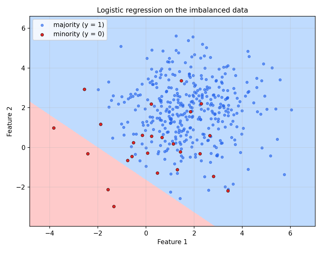
The line has been pushed into the far corner. The model is working hard to avoid any mistakes on the blue majority points and has effectively given up on the red ones: only 4 of the 25 minority points fall on the minority side.
3. Why This Topic Is Worth Your Time
Two reasons, one practical and one career-related.
Imbalanced data is everywhere in industry. Look at where classical machine learning is most heavily used, and at a typical problem in each domain:
| Domain | Typical problem | Rare class |
|---|---|---|
| Finance | Credit card fraud detection | Fraudulent transactions |
| Finance | Credit risk assessment | Borrowers who default |
| Healthcare | Rare disease prediction | Patients who have the disease |
| Manufacturing | Predicting machine failure | Machines about to fail |
| Consumer internet | Churn prediction (Netflix, Amazon Prime) | Customers who'll leave next month |
| Environmental science | Earthquake or eruption prediction | Days an event happens |
Every one of these is an imbalanced problem. And in every one of them, the rare class is the one that matters: the fraudulent transaction, the defaulter, the patient with the disease. A model that ignores the minority class here isn't slightly worse, it's useless for the job it was built for.
It comes up in interviews a lot. Because so much real work involves imbalanced data, interviewers use it to check whether a candidate has dealt with real problems rather than just textbook algorithms.
4. The Setup for Every Technique Below
The five techniques that follow all start from the same data and the same split. The imbalanced-learn library (imported as imblearn) implements all the resampling methods and works with scikit-learn's API.
One deliberate change from the source notebook: it uses test_size=0.3 for the baseline but test_size=0.2 for the resampling sections. That makes the results incomparable, and with 0.2 the test set contains only 4 minority points. This post uses test_size=0.3, random_state=42 everywhere, so every technique is scored on the same 120 test points. Even then, that's only 7 minority test points: each one is worth about 14 percentage points of minority recall. Treat the minority-class metrics below as rough indications, not precise measurements.
The training set has 18 minority and 262 majority points.
Every resampling technique below is applied to the training set only. The test set is never resampled, because it has to reflect the real-world class balance the model will face after deployment. Resampling it would make the scores meaningless.
5. Technique 1: Random Undersampling
The problem is that one class has far more points than the other. The most direct fix is to remove points from the majority class until both classes are the same size. With 900 majority and 100 minority points, randomly keep 100 of the 900, and train on the resulting balanced 200.
from imblearn.under_sampling import RandomUnderSampler

rus = RandomUnderSampler(random_state=42)
X_resampled, y_resampled = rus.fit_resample(X_train, y_train)
fit_resample takes the training data and returns a resampled copy. Here X_train has 280 rows (18 minority, 262 majority); X_resampled has 36 rows, 18 of each class.
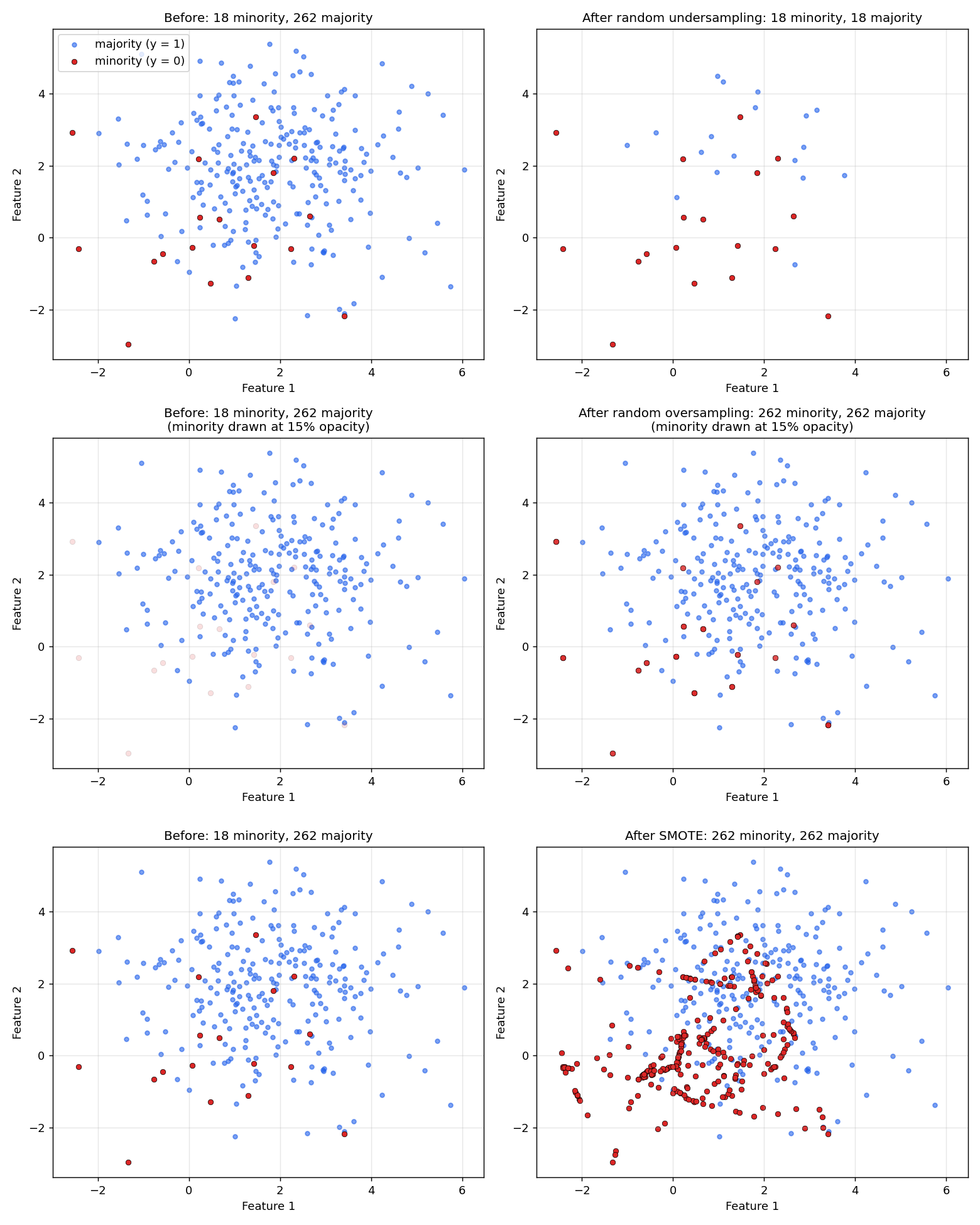
The top row shows what undersampling does: the majority cloud is cut down to 18 points. Training the same logistic regression on this balanced set moves the decision boundary into the middle of the data (see the comparison in Section 8). The minority class is no longer being ignored, because the model now sees as many minority examples as majority ones.
Advantages:
- It reduces the bias toward the majority class. That's the whole point, and the moved boundary confirms it.
- Training gets faster. With 1,000,000 majority rows and 100,000 minority rows, undersampling leaves 200,000 rows to train on instead of 1,100,000.
Disadvantages:
- It throws away a lot of data. Here, 280 training rows become 36. Some of the 244 discarded majority points may have carried information the model needed.
- The random sample itself can be biased. If the kept majority points happen to over-represent one region of the data, the model learns a distorted picture of the majority class. Random sampling usually limits this, but on small data it's a real risk.
6. Technique 2: Random Oversampling
The opposite approach: instead of shrinking the majority, grow the minority. With 900 vs 100, the minority needs 800 more points. Random oversampling gets them in the simplest possible way, by duplicating randomly chosen minority points until the two classes are equal.
from imblearn.over_sampling import RandomOverSampler

ros = RandomOverSampler(random_state=42)
X_resampled, y_resampled = ros.fit_resample(X_train, y_train)
The result has 524 rows: 262 of each class. Look back at the middle row of the figure above. Drawn normally, the "after" plot would look identical to the "before" plot: the same 18 red positions, no new ones. That's because there are no new positions. The 18 original minority points have been copied between 9 and 21 times each (14.6 on average), and the copies sit exactly on top of each other. Drawing the red points at 15% opacity reveals the stacking: a single point is barely visible, while a stack of 15 copies looks solid.
Training on the oversampled data moves the boundary toward the middle, much like undersampling.
Disadvantages:
- The dataset gets bigger. Here it nearly doubles, 280 rows to 524. On a dataset that's already 1 GB, that can mean 2 GB.
- Duplicates encourage overfitting. A point repeated 20 times looks 20 times as important to the learning algorithm. Models that can memorize individual points, decision trees especially, will carve out tiny regions around each duplicated point. That fits the training data well and generalizes badly.
7. Technique 3: SMOTE
SMOTE (Synthetic Minority Oversampling Technique) is probably the best-known technique for imbalanced data. It's still oversampling, growing the minority class until it matches the majority, but it attacks oversampling's duplication problem directly: instead of copying existing minority points, it generates new, synthetic ones that are similar but not identical. Balance is reached without stacking copies, so the overfitting risk drops.
The new points come from interpolation: each synthetic point is placed somewhere on the straight line between two existing minority points that are close to each other. Step by step:
- Find neighbors. Train a K-nearest-neighbors model on the minority class alone (by default, ), so every minority point knows its 5 closest minority neighbors.
- Pick a point. Choose one minority point at random; call it the original sample.
- Pick a neighbor. Choose one of its 5 neighbors at random.
- Interpolate. Choose a random factor between 0 and 1, and create the new point:
- Repeat steps 2 to 4 until the minority class is as large as the majority.
A small example makes the formula concrete. Say the original sample is , the neighbor is , and :
With , the new point lands exactly halfway between the two. would reproduce the original sample, and would land on the neighbor; anything in between lands on the line segment joining them.
Here's one actual step on the real training data, using the 18 minority training points:
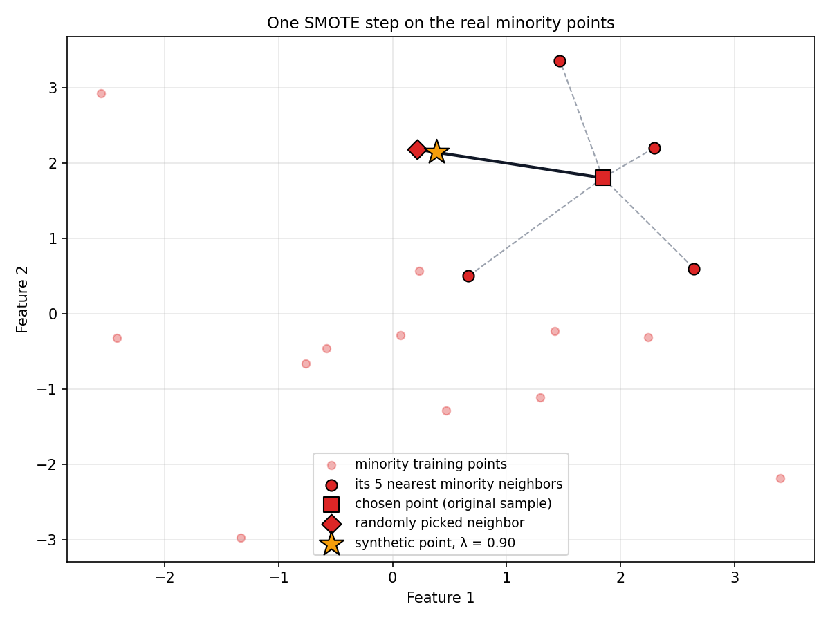
The chosen sample is and the picked neighbor is . With , the formula gives : on the line between them, 90% of the way toward the neighbor.
In code it's the same pattern as before:
from imblearn.over_sampling import SMOTE

smote = SMOTE(random_state=42)
X_resampled_smote, y_resampled_smote = smote.fit_resample(X_train, y_train)
This gives 524 rows, 262 per class, the same counts as random oversampling. The difference is in the bottom row of the before/after figure: this time there are 244 genuinely new red points, laid out along straight lines between the original ones. That straight-line pattern is SMOTE's interpolation, visible directly.
Advantages: it reduces the bias like the other techniques, and since nothing is duplicated, it avoids random oversampling's main overfitting risk.
Disadvantages. SMOTE is popular, but whether to use it at all is genuinely debated, and these are the reasons:
- It can't handle categorical features. Suppose one feature is a category encoded as 0, 1 or 2. Interpolating between a point with value 0 and a point with value 1 can produce 0.7, which isn't a valid category. Plain SMOTE assumes every feature is continuous. (imbalanced-learn has a variant,
SMOTENC, built for mixed numeric and categorical data.) - It's computationally expensive. It runs K-nearest neighbors first, which means computing distances between many pairs of points. On large or high-dimensional datasets, that gets slow.
- Its results depend heavily on . With , every point only ever interpolates toward its single nearest neighbor, so the synthetic points pile up on a few short lines with little variety. With a very large , points get paired with distant neighbors and synthetic points appear all over the feature space. Somewhere in the middle works best, and finding it isn't easy; is the usual default, but the right value depends on the data.
- It's sensitive to outliers. An isolated minority point far from the rest still gets picked as an original sample, and still gets neighbors. Every interpolation from it lays new synthetic points across the empty space between the outlier and the real cluster, so one noisy point produces many more. The real run shows this: in the SMOTE "after" panel, a chain of five synthetic points runs from the isolated red point near across otherwise empty space toward the main cluster, and several lines cut straight through the dense blue majority region, creating minority points in places where the real data has almost none.
- There's no guarantee the synthetic points are realistic. This is the biggest criticism. Generating thousands of new points is easy; knowing that they actually follow the true distribution of the minority class is not. If they don't, the model is learning from data that doesn't describe reality.
8. What the Three Resampling Techniques Actually Changed
Training the same logistic regression on each resampled training set and plotting its decision boundary:
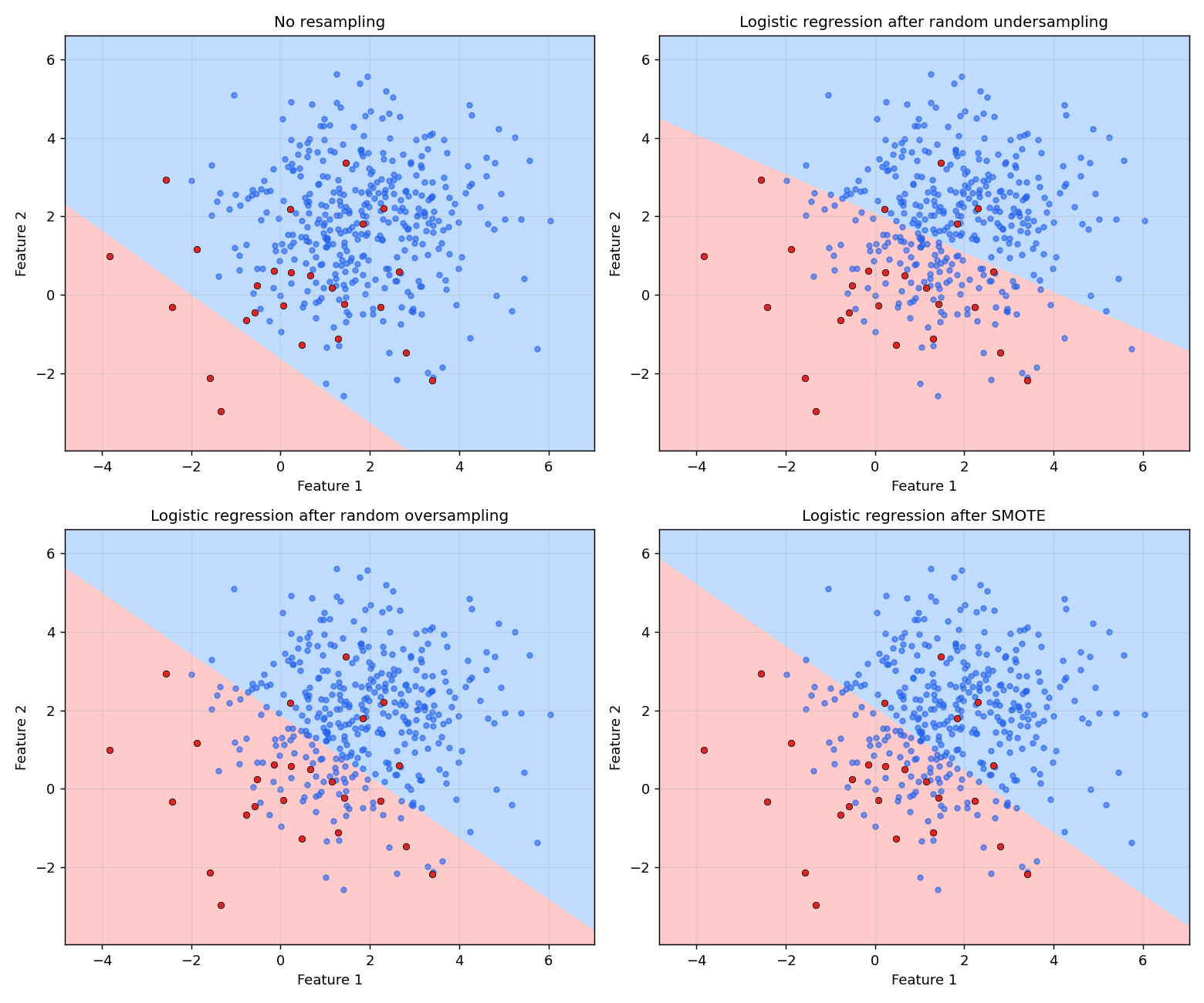
All three move the boundary from the far corner into the middle of the data, so it now gives both classes roughly equal weight. Here are the actual test-set scores, with minority-class (class 0) metrics, on the same 120-point test set:
| Model | Accuracy | Minority recall | Minority precision | Minority F1 | ROC AUC |
|---|---|---|---|---|---|
| Always predict majority | 0.942 | 0.00 (0 of 7) | n/a | 0.00 | 0.500 |
| Logistic regression, no resampling | 0.958 | 0.29 (2 of 7) | 1.00 | 0.44 | 0.956 |
| + random undersampling | 0.617 | 1.00 (7 of 7) | 0.13 | 0.23 | 0.947 |
| + random oversampling | 0.742 | 1.00 (7 of 7) | 0.18 | 0.31 | 0.954 |
| + SMOTE | 0.708 | 1.00 (7 of 7) | 0.17 | 0.29 | 0.954 |
The pattern is consistent: minority recall shoots up, while minority precision and overall accuracy fall. Every resampled model catches all 7 minority test points, but it also flags many majority points as minority (precision 0.13 to 0.18 means only 1 in 6 or 7 minority predictions is right). Whether that trade is worth it depends entirely on the problem: for fraud or rare disease, missing the rare case is usually far more costly than a false alarm, so this trade is often exactly what's wanted.
The results aren't spectacular for a second reason: the data isn't linearly separable. The two blobs overlap heavily, and logistic regression can only draw a straight line. A model that can draw non-linear boundaries, like a random forest or a boosting model, has more room to do better here.
The last column shows something important. ROC AUC barely moves: 0.956 without resampling, 0.947 to 0.954 with it. ROC AUC measures how well the model ranks points, whether minority points tend to get higher minority-probabilities than majority points, independent of any threshold. Resampling hardly changed that ranking. What it mainly changed is where the cut-off sits: by presenting the model with a 50/50 class balance, it shifted the boundary toward the majority class. For a simple linear model like this one, that's most of what these techniques do. They don't give the model new information about the minority class; they change how willing it is to predict it.
9. Technique 4: Ensemble Methods (Balanced Random Forest)
Ensemble methods like bagging, random forests and boosting can be tweaked to handle imbalance internally. One example is the balanced random forest.
A normal random forest trains many decision trees, each on its own random sample of the training data, and combines their votes. A balanced random forest changes just one thing: each tree's sample is drawn so that it's balanced. With 900 majority and 300 minority points, the first tree might get the 300 minority points plus a random 300 of the majority; the second tree gets the minority points plus a different random 300 of the majority; and so on. Every tree trains on balanced data, yet across all the trees, most of the majority class gets used somewhere. That avoids undersampling's biggest weakness, throwing data away, while still giving each tree a balanced view. (imbalanced-learn's current implementation also draws the minority points with replacement, so each tree sees a slightly different set of those too.) Prediction works as in any random forest: each tree votes and the majority vote wins, for example two trees voting 1 and one voting 0 gives 1.
No separate resampling step is needed; the balancing happens inside the model:
from imblearn.ensemble import BalancedRandomForestClassifier

classifier = BalancedRandomForestClassifier(random_state=42)
classifier.fit(X_train, y_train)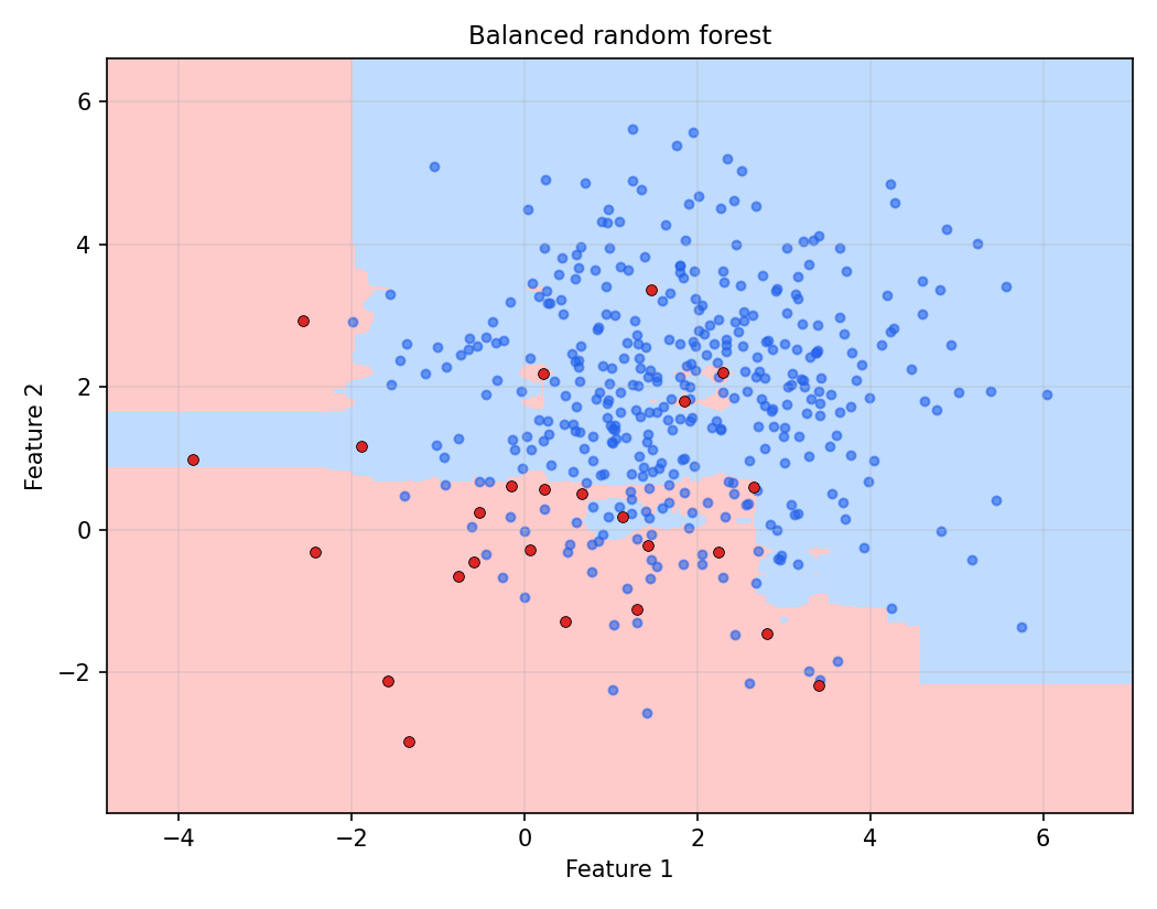
Unlike logistic regression's straight line, the boundary is non-linear, built from the trees' axis-aligned splits, and it wraps around regions where the minority points are. On the test set: accuracy 0.792, minority recall 0.57 (4 of 7), minority precision 0.15, ROC AUC 0.832. Recall improved over the baseline's 0.29, precision is low, and ROC AUC is actually lower than logistic regression's, which isn't surprising for a fully grown forest on 18 minority points with no tuning at all. Tuning tree depth and the number of trees would likely help. Boosting algorithms can be adapted the same way.
10. Technique 5: Cost-Sensitive Learning
The previous techniques changed the data the model sees. Cost-sensitive learning leaves the data alone and changes the learning process, so that mistakes on the minority class cost the model more. Two ways to do it.
Class weights
Assign each class a weight, and make the minority class's weight larger. If class 1 is the majority (900 points) and class 0 the minority (100 points), you might give class 0 a weight of 10 and class 1 a weight of 1. That tells the algorithm: an error on a class-0 point is 10 times as serious as an error on a class-1 point.
For logistic regression, this means each point's term in the log loss gets multiplied by its class's weight :
During gradient descent, a misclassified minority point now contributes a gradient 10 times larger, so the parameter update it causes is 10 times larger, and the model moves much more strongly to fix minority-class mistakes. In effect, the 100 minority points pull on the model about as hard as the 900 majority points do, without a single row being added or removed.
Most scikit-learn classifiers support this through a class_weight parameter, including LogisticRegression, SVC, DecisionTreeClassifier and random forests, and boosting libraries offer equivalents. Algorithms without a loss function to weight don't: KNeighborsClassifier and the naive Bayes classifiers have no class_weight. Using it is a single argument:
model = LogisticRegression(class_weight={0: 50, 1: 1}, solver='liblinear')
model.fit(X_train, y_train)
Turning the minority weight up step by step shows exactly what it does:
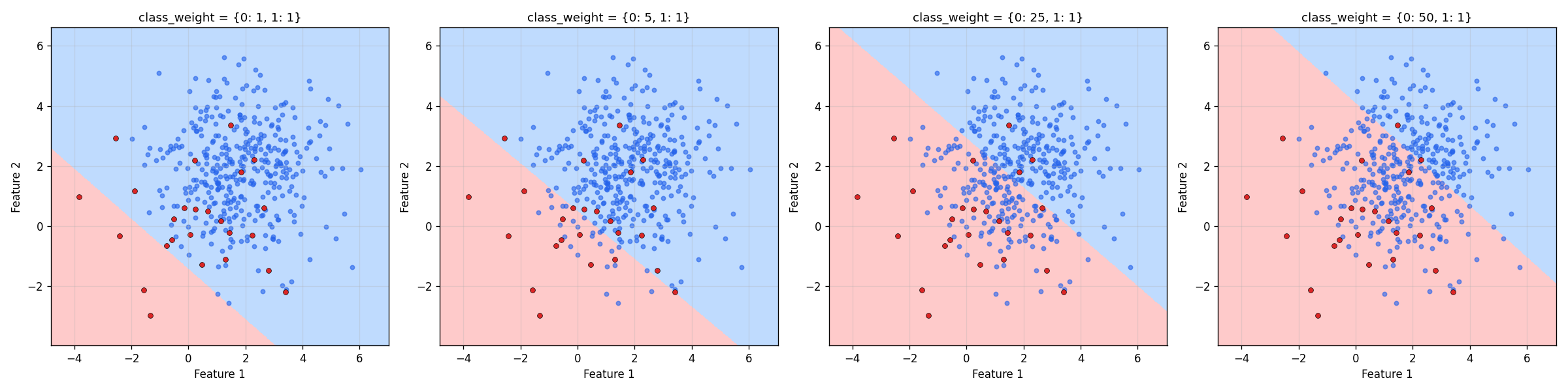
class_weight for class 0 | Accuracy | Minority recall | Minority precision | ROC AUC |
|---|---|---|---|---|
| 1 (no weighting) | 0.958 | 0.29 (2 of 7) | 1.00 | 0.954 |
| 5 | 0.917 | 0.71 (5 of 7) | 0.38 | 0.954 |
| 25 | 0.583 | 1.00 (7 of 7) | 0.12 | 0.956 |
| 50 | 0.408 | 1.00 (7 of 7) | 0.09 | 0.953 |
The weight works like a dial. More weight pushes the boundary further into the majority class, increasing recall and lowering precision. A weight of 5 gives the best balance in this table, with minority F1 0.50, higher than any resampling technique in Section 8. A weight of 50 overshoots: every minority point is caught, but only 41% of all predictions are right. As with resampling, ROC AUC stays flat at about 0.95, because weighting moves the boundary rather than changing how the model ranks points. Rather than guessing, class_weight='balanced' sets each class's weight to (for training rows and rows in class ), which here gives class 0 a weight of 7.78 and class 1 a weight of 0.53. It's a sensible starting point to tune from.
One correction relative to the source notebook: its class-weights cell computes ROC AUC with classifier.predict_proba, the balanced random forest from the previous section, instead of the weighted logistic regression model. The AUC values above are computed from the correct model.
A custom loss function
Some algorithms, particularly boosting libraries like XGBoost, LightGBM and gradient boosting, let you pass your own loss function. That allows any trade-off to be encoded directly: for example, making one kind of error more costly than the other. The source notebook does this with XGBoost:
import xgboost as xgb

def custom_loss(preds, dtrain):
    labels = dtrain.get_label()
    preds = 1.0 / (1.0 + np.exp(-preds))  # Convert to probability

    # Define penalties
    false_positive_penalty = 10
    false_negative_penalty = 1.0

    grad = (preds - labels) * ((labels == 1) * false_negative_penalty + (labels == 0) * false_positive_penalty)
    hess = preds * (1 - preds) * ((labels == 1) * false_negative_penalty + (labels == 0) * false_positive_penalty)
    return grad, hess

dtrain = xgb.DMatrix(X_train, label=y_train)
dtest = xgb.DMatrix(X_test, label=y_test)

params = {'max_depth': 3, 'eta': 0.1}
bst = xgb.train(params, dtrain, num_boost_round=10, obj=custom_loss)
XGBoost needs two things from a custom loss: its gradient and its Hessian (second derivative) with respect to the model's raw score, for every row. That's what custom_loss returns. Comparing it with the weighted log loss above: for log loss, the gradient with respect to the raw score is and the Hessian is . Multiply both by a per-row weight and you get exactly these two lines. So this custom loss is weighted log loss: class-weighting, implemented by hand for XGBoost.
The names "false positive" and "false negative" need care here. In this setup, label 1 (the majority) is the "positive" class. A false positive is a row whose true label is 0, the minority, that the model predicted as 1. So false_positive_penalty is the weight on every minority row's error, and raising it to 10 is the same thing as giving the minority class a class weight of 10. That framing fits problems where false positives are the critical error, like a spam filter, where flagging a genuine email as spam is worse than letting one spam message through.
One more correction. The notebook converts predictions to classes with bst.predict(dtest) > 0.5. With a custom objective, XGBoost doesn't know what transformation the loss applies, so predict returns raw scores (log-odds), not probabilities. A probability of 0.5 corresponds to a raw score of 0, so the correct threshold is > 0; thresholding raw scores at 0.5 is actually a probability cut-off of about 0.62. The charts and numbers here use > 0. (The 'silent' parameter in the notebook's params has also been dropped, since current XGBoost ignores it and only prints a warning.)
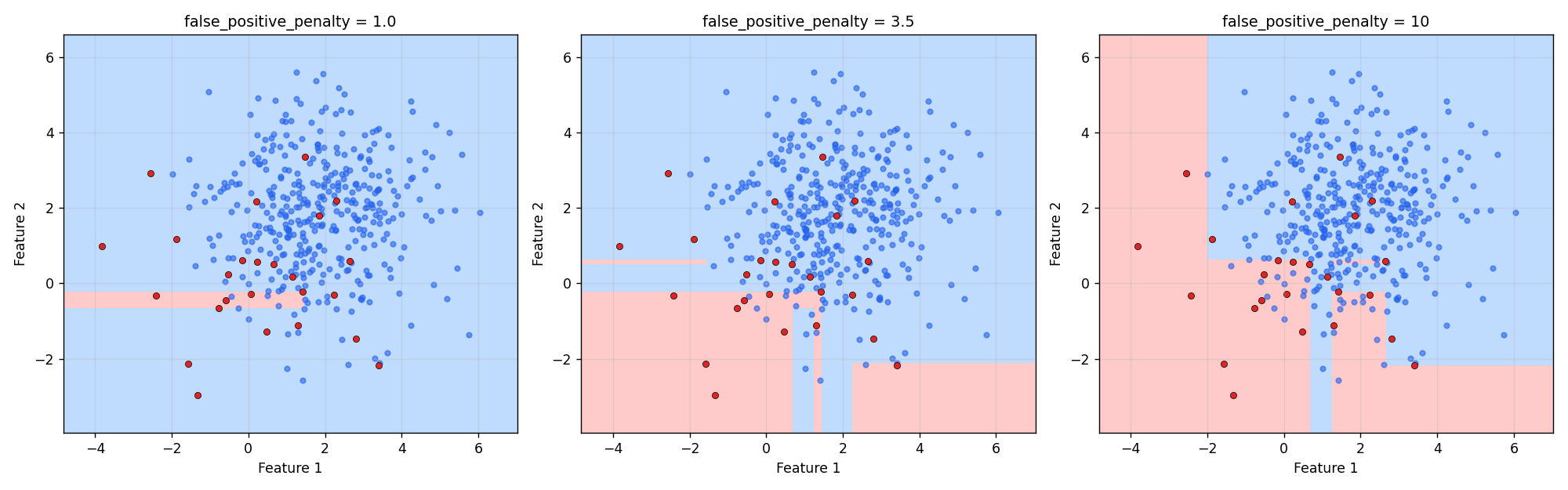
false_positive_penalty | Accuracy | Minority recall | Minority precision | ROC AUC |
|---|---|---|---|---|
| 1.0 (plain log loss) | 0.917 | 0.00 (0 of 7) | 0.00 | 0.904 |
| 3.5 | 0.908 | 0.14 (1 of 7) | 0.17 | 0.898 |
| 10 | 0.875 | 0.57 (4 of 7) | 0.25 | 0.732 |
With no extra penalty, these 10 shallow trees never predict the minority class on the test set. Raising the penalty grows the predicted-minority region (the blocky shapes come from the trees' axis-aligned splits) and recall rises accordingly. Plain class weights are usually the easier way to get the same effect: XGBoost supports per-row weights in DMatrix and a scale_pos_weight parameter. A custom loss is worth the extra effort when the cost structure is something weights can't express.
11. Other Techniques
The five above are the most common, but the imbalanced-learn API reference lists many more, and it's worth browsing:
- Smarter undersampling:
TomekLinks,NearMissandEditedNearestNeighbourschoose which majority points to remove (for example, ones right on the class boundary) instead of removing them at random. - SMOTE variants:
BorderlineSMOTEandSVMSMOTEconcentrate synthetic points near the class boundary,ADASYNgenerates more of them where the minority class is hardest to learn, andSMOTENChandles mixed numeric and categorical features. - Combinations:
SMOTETomekandSMOTEENNoversample with SMOTE, then clean up noisy points with an undersampler. - Ensembles: besides
BalancedRandomForestClassifier, there areBalancedBaggingClassifier,EasyEnsembleClassifierandRUSBoostClassifier.
12. What to Take Away
- Imbalanced data means one class vastly outnumbers another. It's the norm, not the exception, in fraud, credit risk, disease prediction, failure prediction and churn, and in nearly all of them the rare class is the one that matters.
- It causes two problems: the model becomes biased toward the majority class, and accuracy becomes misleading. Here, 96% accuracy came with only 2 of 7 minority points caught, against 94.2% for a model that never predicts the minority at all. Look at per-class recall, precision, F1 and ROC AUC instead.
- Random undersampling removes majority points (fast, but discards data). Random oversampling duplicates minority points (no data lost, but bigger data and overfitting risk). SMOTE creates synthetic minority points by interpolating between neighbors, , which avoids duplication but can't handle categorical features, depends on , amplifies outliers, and can generate unrealistic points.
- Balanced random forest gives each tree a balanced sample, so each tree is balanced without discarding data overall. Cost-sensitive learning leaves the data alone and makes minority errors cost more, through
class_weightor a custom loss. - Resample only the training data, never the test set.
- On this dataset, every technique traded precision for recall while ROC AUC barely moved: they mostly moved the decision boundary rather than teaching the model anything new. The right setting depends on how costly a missed minority case is compared to a false alarm in your problem.