Ch.58: Gradient Boosting, the Regression Intuition

By Ayush Arora•2026-09-26•8 min read

Inspired by: YouTube

Gradient boosting is a boosting algorithm, same family as AdaBoost: small models added one at a time, each one aware of what the ones before it got wrong. What changes is how that awareness gets passed forward. AdaBoost reweights rows so the next stump pays more attention to the ones it missed. Gradient boosting takes a more direct route: it hands the next model the previous model's error itself, as a number to predict. This post covers the regression case and stays at the intuition level, exactly how the source video sequences it; the math behind why this works is deferred to a follow-up post, same as the plan the video itself lays out.

1. Stage 1 Isn't a Model, It's a Number

Ask what the very first "model" in a gradient boosting regressor looks like, and the answer is anticlimactic: it's the mean of the target column. Not a tree, not a linear fit, just a single number that gets returned for every row regardless of its features.

Take a toy dataset of 5 students with a known salary (in LPA): 3, 4, 8, 6, 3. Stage 1's prediction for every student, no matter their IQ or CGPA, is:

\text{model}_1 = \frac{3+4+8+6+3}{5} = 4.8

That's it. Why the mean specifically, rather than the median or something else, is the subject of the next post's derivation; for now it's enough to know that stage 1 is a constant, and every subsequent stage's whole job is to chip away at how wrong that constant is for each individual row.

2. The Pseudo-Residual: What Gets Passed Forward

Once stage 1 exists, its error per row is just actual minus predicted:

Student	Actual salary	Model 1 prediction	Residual
1	3	4.8	-1.8
2	4	4.8	-0.8
3	8	4.8	3.2
4	6	4.8	1.2
5	3	4.8	-1.8

This is called a pseudo-residual, "pseudo" because it borrows the name from ordinary linear regression's residual ( $y - \hat{y}$ ) without being derived the same way, it's a stand-in for a more general quantity (the negative gradient of the loss function) that the math post will make precise. For now, actual minus predicted is the working definition.

3. Stage 2 Predicts the Error, Not the Salary

Here's the part that's easy to get backwards: stage 2 is a decision tree trained on the same input features (IQ, CGPA), but its target column is the residual, not the salary. You're not asking "what's this student's salary", you're asking "how wrong was stage 1 for this student, based on their IQ and CGPA". If stage 2 gets good at predicting that, the combined model (stage 1 + stage 2) automatically gets better at predicting the actual salary, without stage 2 ever being told what a salary is.

With this toy dataset small enough for a tree to fit exactly, stage 2 reproduces each row's residual perfectly. That means stage 1 + stage 2 reproduces the training salaries exactly too: 4.8 + (-1.8) = 3, 4.8 + (-0.8) = 4, matching the actual values row for row. That looks like a win, but it's actually a warning sign: a model that reproduces its training data exactly is overfitting, it will do the same thing on a brand-new student it hasn't seen and get it badly wrong, since real data won't hand it the exact residual to add back.

4. The Fix: a Shared Learning Rate

Gradient boosting's answer to that overfitting is a learning rate, typically 0.1, that scales down every stage after the first:

\hat{y} = \text{model}_1 + \eta \cdot \text{model}_2 + \eta \cdot \text{model}_3 + \dots

With $\eta = 0.1$ instead of the implicit 1 from the previous section, student 1's prediction becomes $4.8 + 0.1 \times (-1.8) = 4.62$ instead of exactly 3. That's a much smaller, more cautious step toward the actual value. The next stage's residual is now $3 - 4.62 = -1.62$ , still nonzero (as opposed to the 0 you'd get from a full step), but visibly closer to 0 than the original -1.8. Recomputing this over the whole toy set: residual 1 → residual 2 goes -1.8 → -1.62, -0.8 → -0.72, 3.2 → 2.88, each row's error shrinking a little, not vanishing all at once.

That's the whole training loop: fit a tree on the current residual, take a small step in that tree's direction (scaled by $\eta$ ), recompute the residual, repeat. More stages push every residual closer to 0 gradually rather than any single stage jumping straight to a perfect (and overfit) fit. The learning rate is the same number for every stage, unlike AdaBoost's α, which is computed fresh per stage based on how good that specific stump was. Gradient boosting's stages all get the same discount; what changes stage to stage is what each stage is trying to correct, not how much it's trusted.

5. Seeing It Converge on Real Data

The toy dataset above is small enough to overfit almost immediately, which makes the mechanism clear but doesn't show the gradual convergence very well. For that, here's the same procedure on a synthetic 100-row dataset from the source notebook ( $y = 3x^2$ plus noise, a curve no single stump could fit well), run with learning_rate = 1 (matching the notebook) and max_leaf_nodes = 8 per tree:

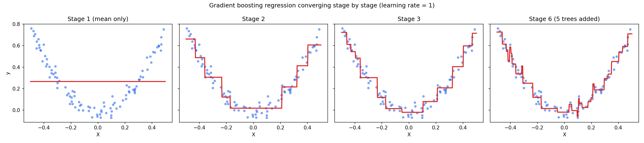
Four scatter plots of the same 100-point noisy quadratic dataset (X from -0.5 to 0.5, y a U-shaped curve). Stage 1 shows a flat red line at the mean, y approximately 0.27, fitting nothing. Stage 2 shows a red step function loosely tracing the U-shape after one tree is added. Stage 3 tracks the curve more closely with finer steps. Stage 6 (after 5 trees total) hugs the U-shape closely, including a small sharp upward spike near X=0.1 where one tree overfit a single noisy point.

Each added tree tightens the fit around the true curve. Worth being honest about the last panel: that sharp spike near $X=0.1$ isn't a bug in the code, it's a real tree deciding a single noisy point deserved its own leaf, an early sign of exactly the overfitting Section 3 warned about, showing up on real (if small) data instead of just the toy example.

6. Why the Learning Rate Actually Matters

Section 4 argued for a smaller learning rate in the abstract; here's what it costs concretely. Running the same 100-row dataset for the same 5 added trees, once with learning_rate = 1 and once with learning_rate = 0.1:

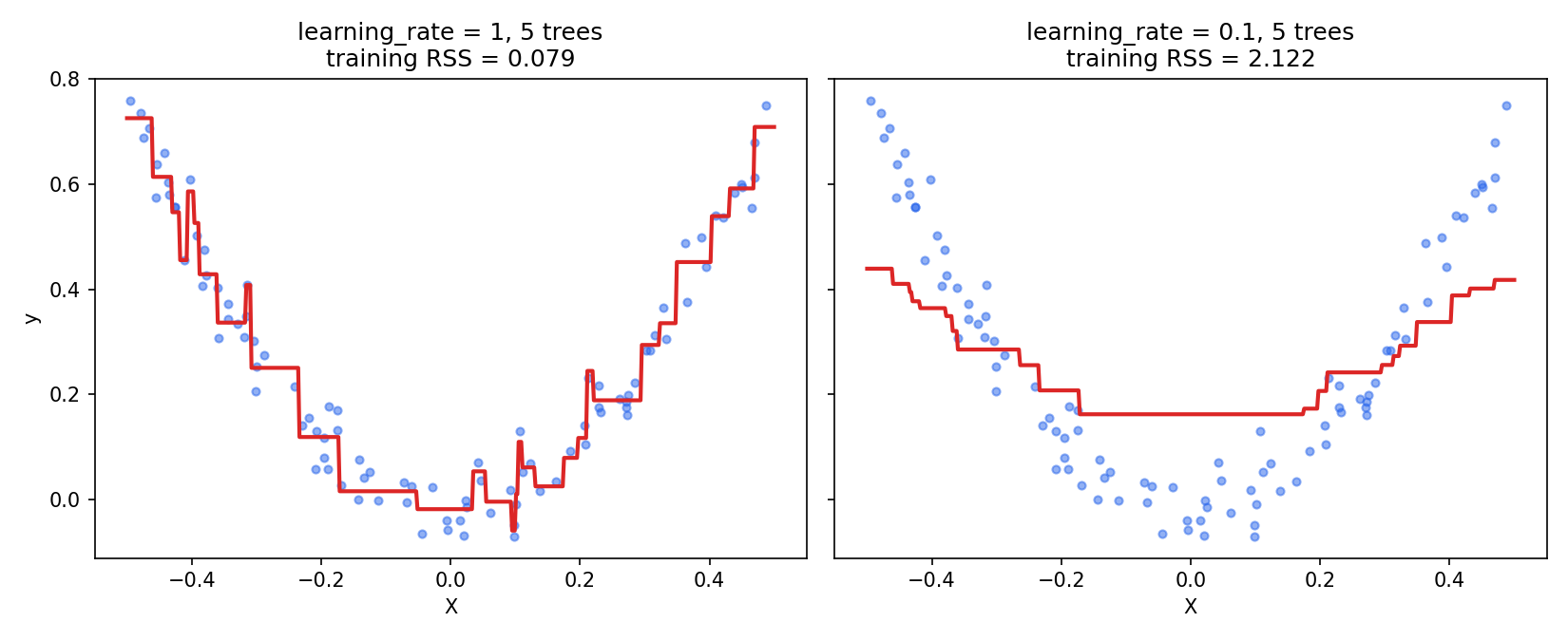
Two scatter plots side by side of the same quadratic dataset with 5 trees added. Left, learning rate 1, the red fitted curve hugs the U-shape tightly, training residual sum of squares 0.079, including the same overfitting spike near X=0.1. Right, learning rate 0.1, the red fitted curve is much flatter and further from the U-shape, training residual sum of squares 2.122, clearly underfit after only 5 stages.

At learning_rate = 1, 5 trees are already enough to hug the training data tightly, overfitting spike included. At learning_rate = 0.1, those same 5 trees have only taken small steps and are still visibly underfit, training error over 25 times higher. Neither is "correct" in isolation, a small learning rate needs many more stages to reach the same fit a large one reaches quickly, which is exactly the trade-off the video points at: smaller steps in the right direction, more of them, rather than one big step that overshoots into memorization.

7. Gradient Boosting vs. AdaBoost: Two Concrete Differences

With both algorithms now covered, the contrast is specific, not just "both do boosting":

Tree size. AdaBoost uses decision stumps, max_depth = 1. Gradient boosting uses noticeably bigger trees, typically max_leaf_nodes between 8 and 32 (8 was used above, since the dataset is small).
Per-stage weighting. AdaBoost computes a distinct α per stage from that stage's error rate, some stumps count more than others in the final vote. Gradient boosting uses one shared learning rate across every stage; no stage is individually up- or down-weighted relative to the others, the only thing that changes between stages is what target (which residual) each one is trained on.

8. What to Take Away

Stage 1 of a gradient boosting regressor is just the mean of the target column, not a trained model.
Every later stage is a tree trained to predict the current residual (actual minus the ensemble's prediction so far), not the original target.
Final prediction is $\text{model}_1 + \eta \sum \text{model}_i$ for $i \geq 2$ , with the same $\eta$ applied to every stage.
Without a learning rate below 1, a tree can fit the training residuals so well that the combined model reproduces the training targets exactly, a clear overfitting signal, not a good outcome.
A smaller learning rate needs more stages to reach the same fit; it trades training speed for a path that's less likely to memorize noise along the way.
The next post works out the math for why the mean and the residual are the right choices, not just useful ones.

View all chapters in Machine Learning Algorithms →