Ch.59: Gradient Boosting Regression, the Actual Math

Inspired by: YouTube

The previous post covered gradient boosting's regression procedure but deferred every "why": why the first model is the mean, why the target that gets passed forward is called a pseudo-residual instead of a plain residual, and why a fitted tree's leaf values line up so neatly with what the algorithm needs. All three turn out to be the same differentiation, applied three times to the same loss function. This post works through it, following Friedman's original gradient boosting algorithm, and checks every number against a real, tiny dataset along the way.

1. Additive Modeling: Why Add Small Functions at All

Machine learning, stripped down, is finding a function $f$ that maps inputs to an output: $y = f(x)$. Sometimes that function is simple enough for one model, a straight line, a polynomial. But some relationships are genuinely composite, built out of several simpler functions added together. A toy example: $f(x) = x + \sin(x)$ is not something a single straight line or a single low-degree polynomial captures well, but it's exactly the sum of two functions that are individually easy to reason about.

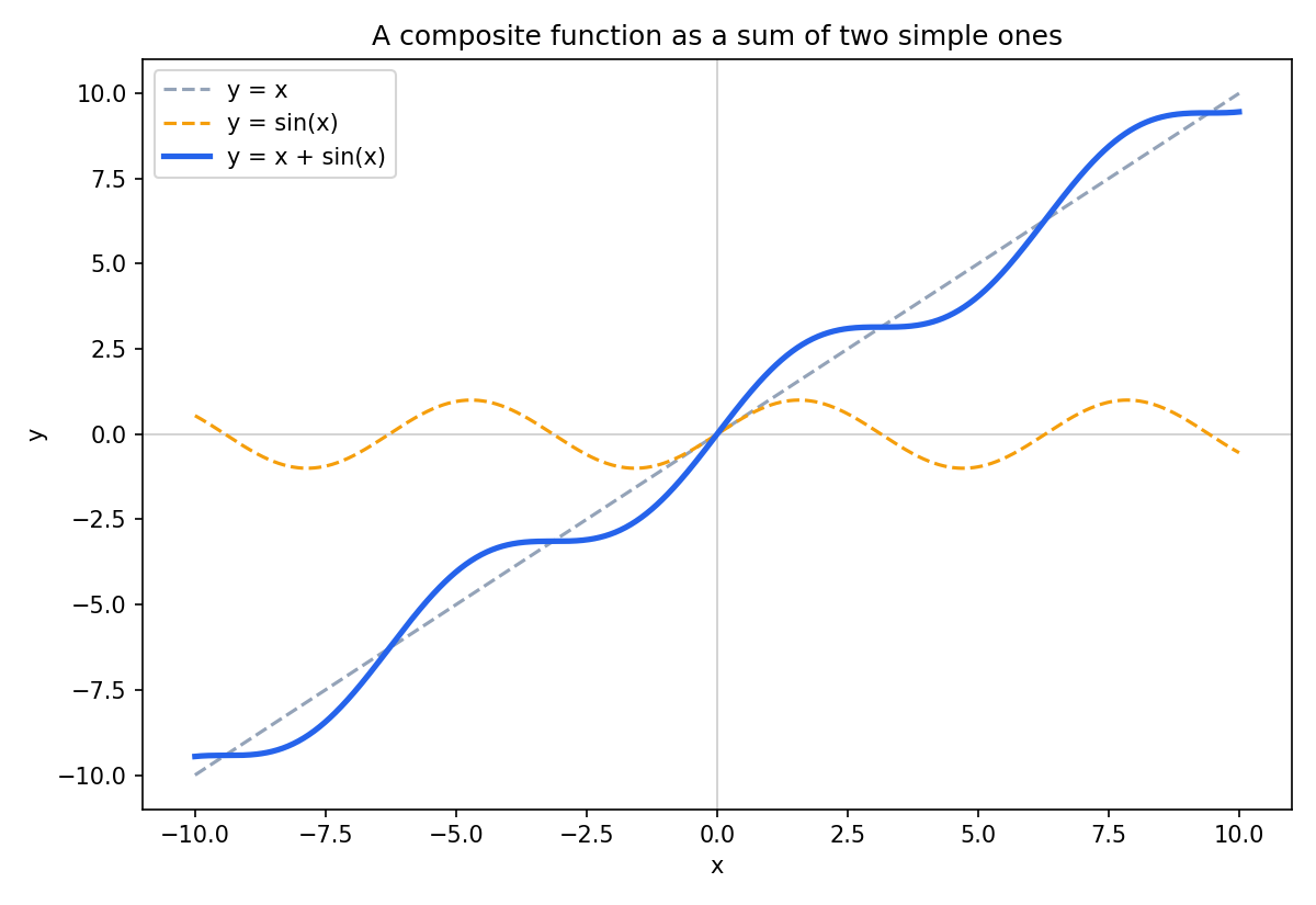
The blue curve is genuinely hard to describe as "one simple shape", it's not a line, not a low-degree polynomial, but it's exactly the straight line plus the sine wave, two shapes that are each trivial on their own. That's the whole idea additive modeling borrows: instead of hunting for one function that matches the blue curve directly, build it by adding simple pieces one at a time.

Additive modeling is the strategy of not trying to find the whole composite function in one shot, and instead building it up piece by piece: fit a small function, see what's left unexplained, fit another small function to explain more of that, and so on. Every boosting algorithm, AdaBoost included, is a specific recipe for doing this. Gradient boosting's version, for regression, is what this post derives.

There's a cautionary reason to prefer "add several simple pieces" over "keep reaching for one increasingly complex function", and it has a name: Runge's phenomenon. If you try to fit a single polynomial through a set of evenly spaced points on a smooth curve, the intuitive expectation is that a higher-degree polynomial, with more terms to work with, should track the curve more closely. In practice it doesn't: past a certain degree, the polynomial starts oscillating wildly near the edges of the interval, and the fitting error near those edges actually gets worse as more terms are added, not better.

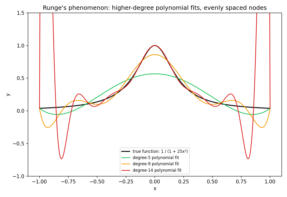
The degree-14 fit matches the true curve almost exactly through the middle, yet near $x = \pm 1$ it swings from roughly $-0.7$ up past $1.5$, wildly overshooting a function that never leaves $[0, 1]$. Adding more polynomial terms didn't buy a better fit everywhere, it bought a worse one at the edges. It's a concrete demonstration that "more complex" and "better fit" aren't the same thing for a single function, which is exactly the failure mode additive modeling sidesteps: instead of cranking up the complexity of one function until it breaks, keep every individual piece small and well-behaved, and let the sum of many simple pieces do the work a single complicated one can't do reliably.

2. What Goes In: Data and a Differentiable Loss

The algorithm needs two things: training data $\{(x_i, y_i)\}_{i=1}^n$, and a loss function $L(y, F(x))$ that must be differentiable, since the entire derivation below leans on taking derivatives and setting them to zero. This post uses the simplest one, squared error, with a $\frac{1}{2}$ tacked on purely for algebraic convenience (it cancels a factor of 2 that the chain rule would otherwise introduce, and multiplying every candidate model's loss by the same constant $\frac{1}{2}$ never changes which model has the lowest loss):

The worked example throughout is a tiny 3-row slice of a real startups profit dataset (R&D spend, admin spend, marketing spend as inputs, profit as output, values in thousands): profit is 192, 144, and 91 for the three rows.

3. Step 1: Why $F_0(x)$ Is the Mean

The algorithm's first step defines the starting model as:

Read in words: find the single constant $\gamma$ that minimizes the total loss across every training row, if that constant were the prediction for all of them. To find it, differentiate with respect to $\gamma$ and set to zero:

That's the mean, derived, not assumed. Plugging in the three profit values:

(worth flagging: if you round that to a flat 142 before carrying it forward, as is easy to do by hand, every downstream number below drifts slightly, leaf outputs end up about 0.3 off from what a decision tree would compute precisely. Carrying the full $142.33$ avoids that drift.)

This result is specific to squared-error loss. A different differentiable loss function would produce a different formula in place of "take the mean", the shape of the algorithm (differentiate, set to zero, solve for $\gamma$) stays the same regardless of which loss is plugged in.

4. Step 2a: The Pseudo-Residual Is a Gradient, Not Just a Subtraction

The next stage needs a target to fit a tree on. The algorithm's formula for it is:

This looks intimidating mostly because of notation. Read it as: take the loss function, differentiate it with respect to the model's own output $F(x_i)$ (not with respect to $y_i$, which is fixed data), negate it, and evaluate that at the current model $F_{m-1}$. For squared-error loss:

so the negative of that is:

Actual minus predicted, exactly the familiar residual, but now it's clear why it's called pseudo-residual: it isn't defined as "actual minus predicted" by assumption, it's defined as the negative gradient of the loss, and it only happens to simplify to that familiar subtraction because squared-error loss is the one being used. Swap in a different loss function (as later gradient boosting posts on classification will), and the pseudo-residual becomes some other expression, still the negative gradient, no longer literally $y - \hat{y}$.

For the first stage ($m=1$), using the precise $F_0(x) = 142.33$:

5. Step 2b: Fit a Tree to the Residuals

A regression tree is fit with the original inputs as $X$ and these pseudo-residuals as the target, not the original profit column. Whatever split the tree lands on divides the training rows into terminal regions $R_{j,m}$ (a fancy name for "which leaf a row falls into"). With three rows and a single-split, depth-1 tree, this produces two terminal regions, say $R_{1,1}$ (the row with residual $-51.33$ alone) and $R_{2,1}$ (the other two rows together).

6. Step 2c: Why a Leaf's Value Is Also a Mean

Every terminal region needs its own output value $\gamma_{j,m}$, computed by the same optimization pattern as Section 3, but now restricted to only the rows that fell into that particular region:

For the single-row region $R_{1,1}$ (the row with $y_i = 91$), differentiating with respect to $\gamma$ and setting to zero, following exactly the same steps as Section 3, gives:

That's precisely the pseudo-residual for that row, no surprise, since with one row in the region, "minimize the loss over the region" and "minimize the loss for that one row" are the same problem.

For the two-row region $R_{2,1}$ (rows with $y_i = 192$ and $y_i = 144$), the same differentiation now sums over both rows:

This is the mean of the residuals in that region. And that's exactly what a fitted decision tree already does at every leaf: average the target values of whatever rows land there. That's why, back in the previous post's code, nobody ever computes $\gamma_{j,m}$ by hand, the tree already handed it over as the leaf's prediction. It isn't a coincidence that they match, it's a consequence of the loss function: squared-error loss's optimal constant is always a mean, whether you're solving for the whole dataset's baseline (Section 3) or one leaf's correction (this section). A different loss function would make the tree's raw leaf output and the algorithm's actual required $\gamma_{j,m}$ diverge, at which point you would need to explicitly recompute the leaf values rather than trust the tree's own averaging.

7. Step 2d: Updating the Model

The last piece per stage is almost anticlimactic after the derivation above. Written precisely, using an indicator function $I(x \in R_{j,m})$ that's 1 when $x$ falls in that region and 0 otherwise (so that only the matching leaf's $\gamma$ ever gets added for a given row):

In plain terms: whichever leaf a row lands in, add that leaf's $\gamma$ to the running total, every other leaf contributes 0 for that row. Unrolled across stages, $F_1(x) = F_0(x) + \text{tree}_1(x)$, $F_2(x) = F_1(x) + \text{tree}_2(x)$, and so on, which is exactly the additive model from Section 1, now with every term concretely defined. After $M$ stages, the final output is simply $\hat{F}(x) = F_M(x)$, the fully unrolled sum of the mean plus every tree's contribution.

8. What to Take Away

• Additive modeling, approximating a complex function as a sum of simpler ones fit in sequence, is the strategy underneath every boosting algorithm; gradient boosting's regression recipe is one specific instantiation of it.
• $F_0(x)$ being the mean isn't a rule to memorize, it falls out of minimizing squared-error loss over a single constant, via one differentiation.
• The "pseudo" in pseudo-residual signals that it's defined as a loss gradient in general, and only simplifies to a plain subtraction ($y - \hat{y}$) because squared-error loss is the one in use here.
• A fitted regression tree's leaf values already equal the algorithm's required $\gamma_{j,m}$ for squared-error loss, since both are optimized to be the mean of whatever rows fall into that leaf, not a coincidence to be surprised by, a consequence of the loss choice.
• Everything here is loss-function-specific. Swapping the loss changes the formulas for $F_0$, the pseudo-residual, and $\gamma_{j,m}$, while the four-step structure (fit a stage, compute pseudo-residuals, fit a tree to them, solve for each leaf's optimal output) stays fixed. That's the shape classification-flavored gradient boosting will reuse in a later post.