Ch.40: Decision Tree Regression

Inspired by: YouTube

Everything about decision trees so far, the core intuition, entropy and Gini, the hyperparameters, has been about classification: keep splitting until each leaf is (mostly) one class. The same machine predicts continuous numbers too, and only two things change: what a leaf outputs, and how a split is scored.

1. Why Not Just Fit a Line?

A lot of regression problems really are close to linear, marks in an exam against hours of study for a semester, say: study more, generally score more, with plenty of individual scatter around that trend. Linear regression handles that case fine. But push the same idea a little further and it breaks: past some point, more hours stop helping, burnout and diminishing returns start pulling marks back down, and the true relationship rises, then falls. A single straight line can't bend to follow that, it can only split the difference and fit the middle badly in both directions. A decision tree instead cuts the x axis into pieces and predicts a flat value inside each piece, so it can bend with the data as sharply as it needs to.

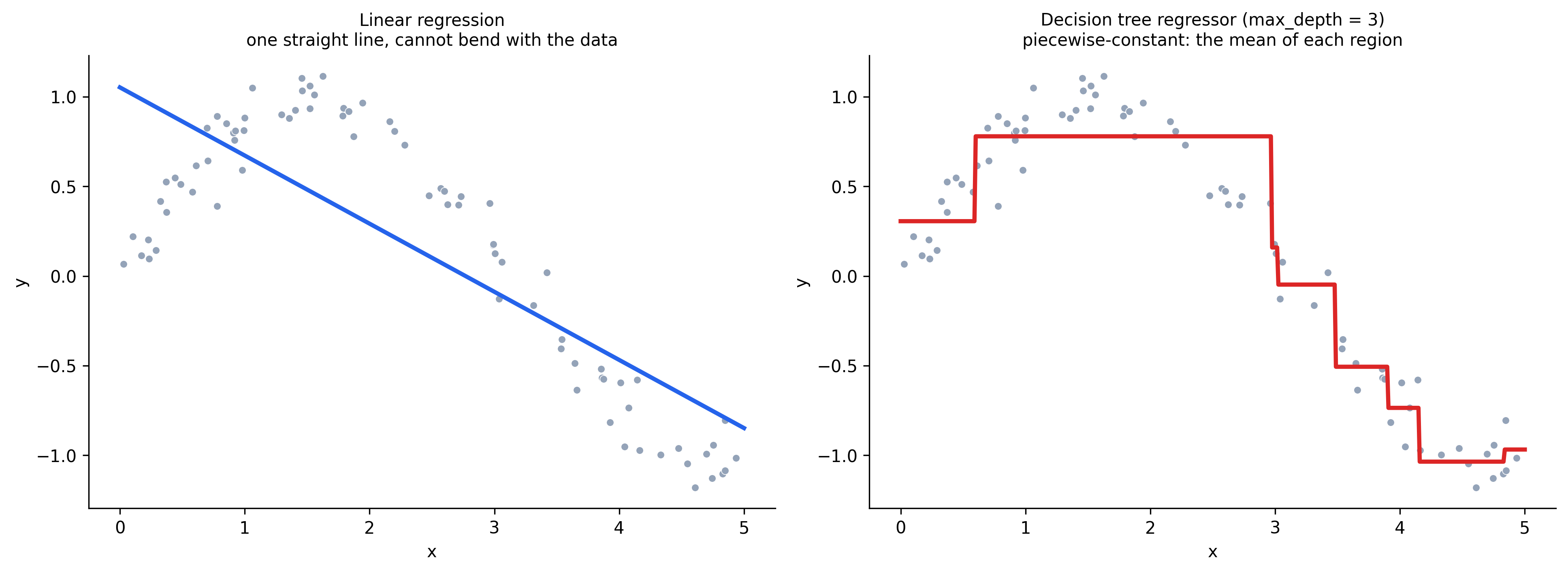
The tree's prediction is a step function: constant within each leaf's region, jumping at the boundaries. With one feature it's a staircase; with two it's a surface of flat rectangular tiles; the idea is the same in any dimension.

2. What a Leaf Predicts

In a classifier, a leaf outputs the majority class of the training rows that landed in it. In a regressor, a leaf outputs their mean target value. If five training points fall into a leaf with targets 3, 4, 4, 5, 9, any new point routed to that leaf gets predicted as 5.0.

That is the whole prediction rule. All the intelligence is in deciding where to cut so that the points sharing a leaf actually have similar targets.

3. How a Split Is Chosen

For classification, ch38 scored a split by how much it reduced Gini impurity or entropy. For regression, the measure is squared error (variance around the mean), and there is no Gini or entropy option at all.

Take the one-feature case. Sort the rows by x, then consider every midpoint between consecutive values as a candidate threshold. For each candidate:

1. Split the rows into a left group (x < threshold) and a right group (x >= threshold).
2. Predict each group's mean.
3. Add up the squared residuals in each group: sum((y_left - mean_left)**2) + sum((y_right - mean_right)**2).

The candidate with the lowest total is the split. (Because the row count is fixed, minimising this sum is the same as minimising the size-weighted mean squared error, which is sklearn's squared_error criterion.)

import numpy as np
 
xs = X.ravel()
midpoints = (np.sort(xs)[:-1] + np.sort(xs)[1:]) / 2
 
best_t, best_sse = None, np.inf
for t in midpoints:
    left, right = y[xs < t], y[xs >= t]
    sse = ((left - left.mean())**2).sum() + ((right - right.mean())**2).sum()
    if sse < best_sse:
        best_t, best_sse = t, sse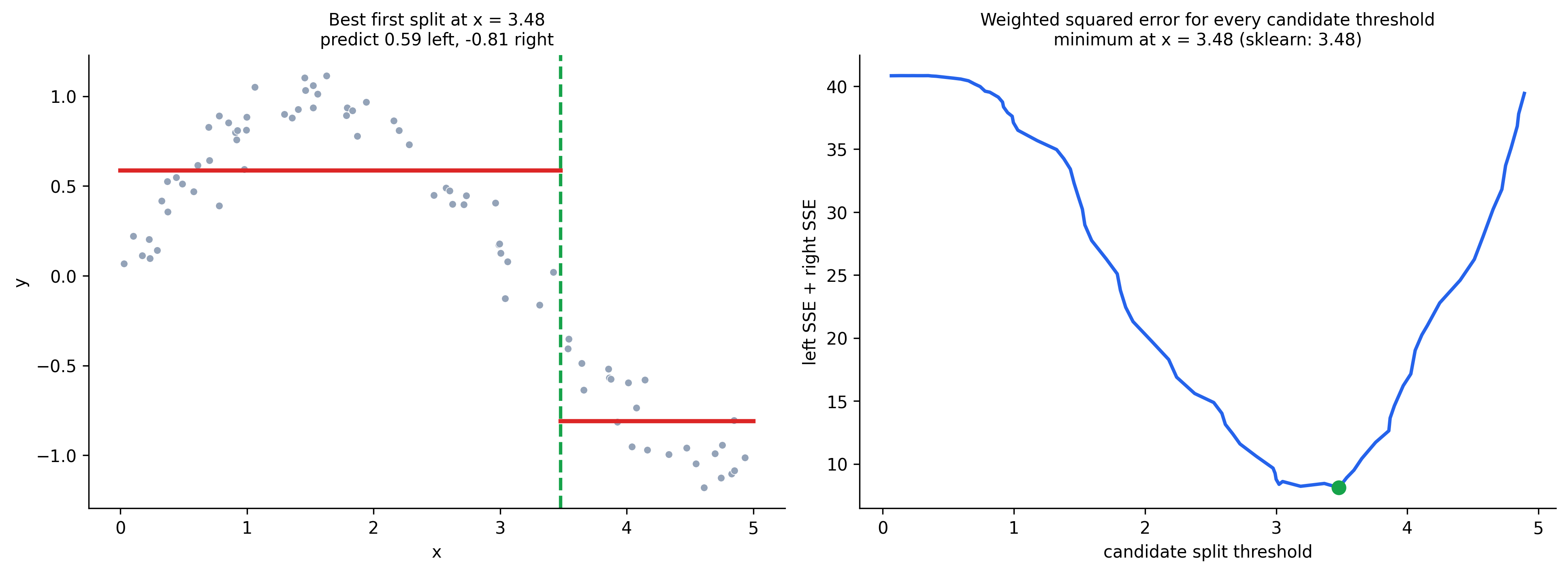

The error curve on the right has a single clear trough: cutting too early (small threshold) or too late (large threshold) leaves one group with a wide spread of targets and a large residual sum. The minimum is where the two groups are internally most alike. A hand-rolled search over midpoints lands on exactly the same threshold sklearn's DecisionTreeRegressor uses for its root split.

Then recurse: run the identical search inside the left region, and again inside the right region, each split shrinking the error a little more.

With more than one feature, a node has to pick which column to cut, not just where. The rule is a direct extension of the single-feature search: run the exact same midpoint sweep independently on every feature, keep each feature's own best (lowest-SSE) threshold, then compare those best-SSE values across features and split on whichever feature reached the lowest one. On load_diabetes, sweeping bmi alone gets its lowest weighted SSE at threshold ≈0.0094 (SSE ≈1.891M); sweeping s5 alone gets ≈1.857M at threshold ≈-0.0038. s5's number is smaller, so the root node splits on s5, exactly the feature and threshold sklearn's DecisionTreeRegressor picks on its own. Every node repeats this feature-vs-feature competition independently, which is why a tree with many input columns can split on a different feature at almost every node.

4. Overfitting Is the Same Story

Left unconstrained, the tree keeps splitting until every leaf holds one training point. Each point then predicts itself, training R² hits a perfect 1.0, and the staircase turns into a spike for every row: a textbook high-variance fit that generalises badly.

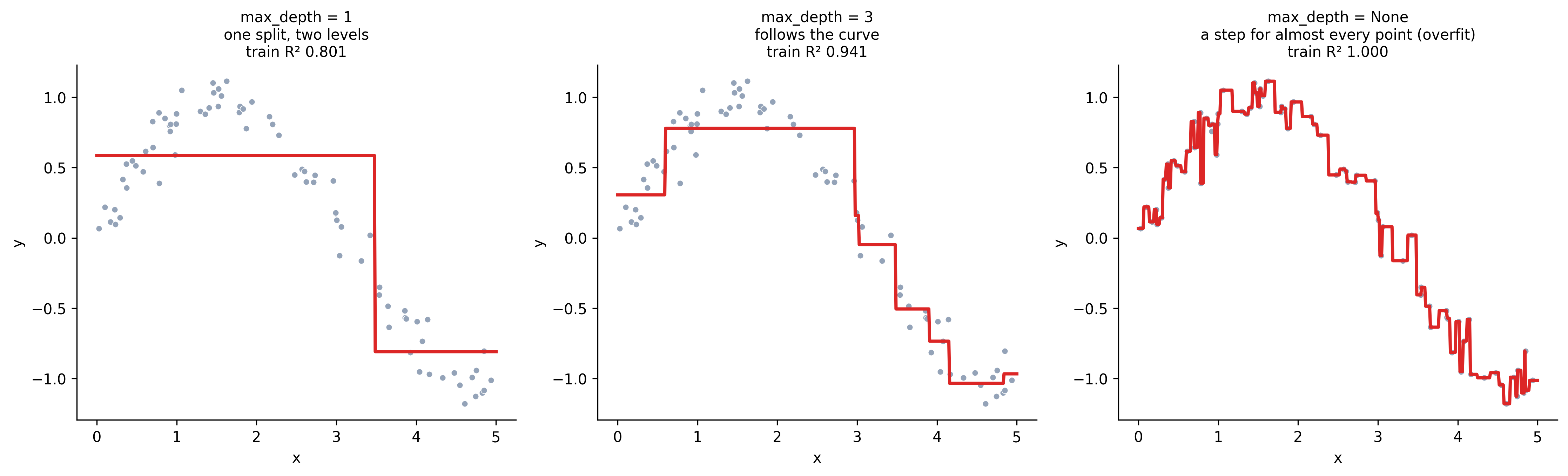
The fix is the same set of stopping controls as the classifier, tuned the same way (compare train against a held-out score, tighten if the gap is wide, loosen if both are low).

5. Hyperparameters That Differ From the Classifier

DecisionTreeRegressor shares almost all of ch39's knobs, with the same meanings: max_depth, min_samples_split, min_samples_leaf, max_leaf_nodes, min_impurity_decrease, max_features, and splitter (best checks every feature and threshold, random picks random thresholds, cheaper and slightly more regularising). Only one thing genuinely changes:

• criterion is squared_error by default (the left-plus-right variance from section 3), with friedman_mse, absolute_error, and poisson as alternatives. gini and entropy do not exist here, they only make sense for classes.

On load_diabetes with max_depth=5 and a fixed train/test split, criterion="squared_error" scores R² ≈ 0.33 on the held-out set against "absolute_error"'s R² ≈ 0.12, a real gap, though not always this size on other data. splitter moves things less: "best" scores the same ≈0.33, "random" comes in at ≈0.34, close enough that the difference is mostly noise here, same as it was for the classifier, with "random" generally the one to reach for if overfitting is the concern.

Everything else transfers directly. max_features has nothing to do on the earlier one-feature toy problem, but on load_diabetes's 10 columns it behaves exactly as it does for the classifier: restricting a node to a random subset of features (half the columns, max_features=5) combined with a tighter min_samples_split (a quarter of the training rows, 88 out of 353) lifts this particular split's test R² from 0.33 to ≈0.39, a concrete case of the general pattern that tighter constraints can help once the unconstrained tree is overfitting.

from sklearn.datasets import load_diabetes
from sklearn.model_selection import train_test_split
from sklearn.tree import DecisionTreeRegressor
from sklearn.metrics import r2_score
 
X, y = load_diabetes(return_X_y=True)
X_train, X_test, y_train, y_test = train_test_split(X, y, test_size=0.2, random_state=42)
 
reg = DecisionTreeRegressor(criterion="squared_error", max_depth=5, random_state=42)
reg.fit(X_train, y_train)
print(r2_score(y_test, reg.predict(X_test)))

A single train/test split like this is noisy, so treat the number as a rough read and use cross_val_score (or the best_score_ from a search) before trusting it. Tuning is the usual GridSearchCV or RandomizedSearchCV over max_depth, criterion, min_samples_split, min_samples_leaf, max_leaf_nodes, and max_features, scoring on cross-validated R².

The explorer below fits a regression tree live on a noisy 1-D wave. Start from the defaults (an unconstrained tree that steps through nearly every point), then set max_depth to 3 or push min_samples_leaf up: the staircase coarsens, train R² drops from a perfect 1.0, and test R² peaks somewhere in between.

6. feature_importances_ and Feature Selection

While building the tree, sklearn tracks how much each split reduces impurity, and adds that up per feature (weighted by how many rows pass through the node), then normalises so the values sum to 1. reg.feature_importances_ exposes the result: a high value means that column carried most of the splitting work.

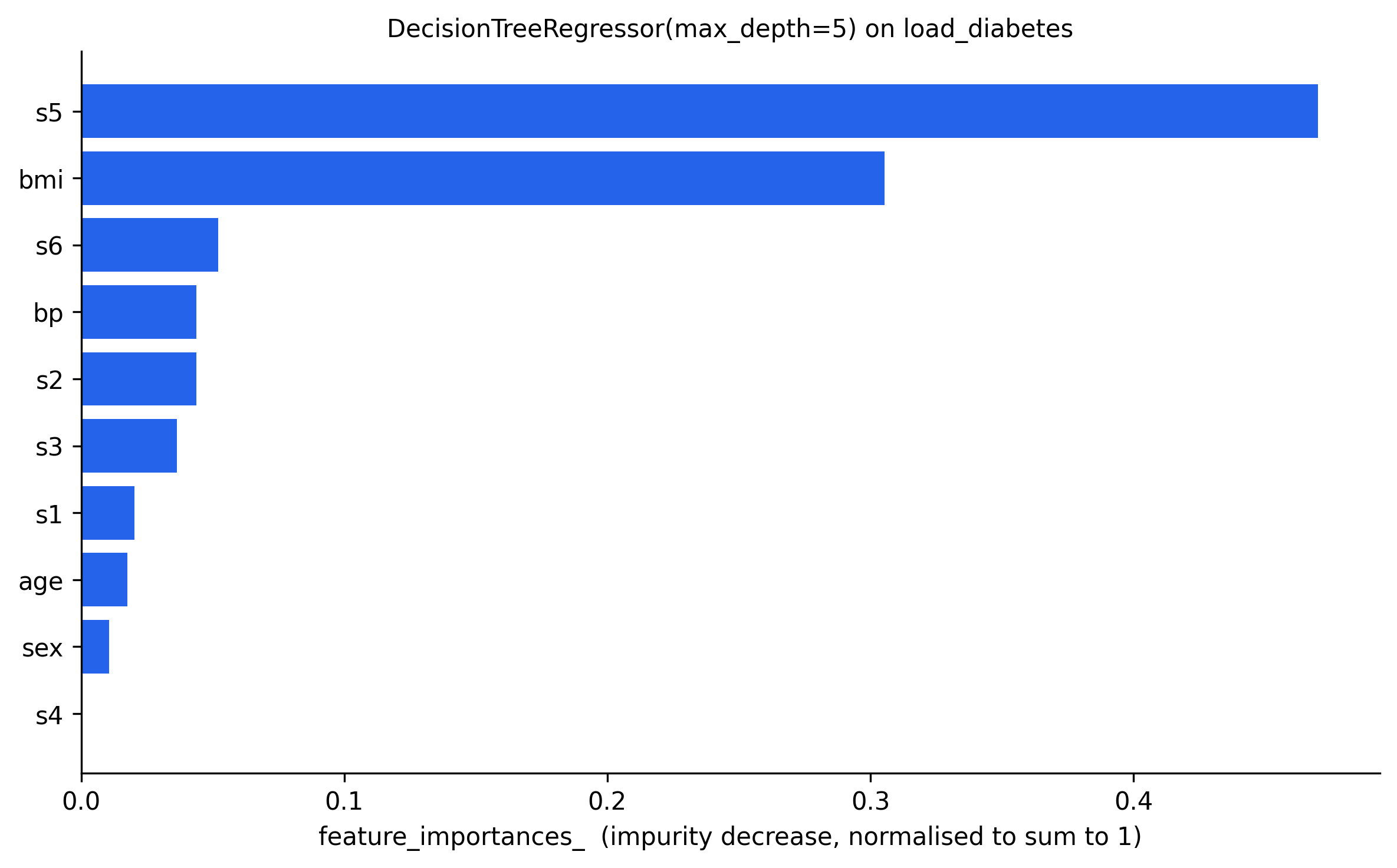
Here two features, s5 and bmi, account for roughly three-quarters of the model, and most of the rest barely move it. That makes this attribute a cheap feature-selection tool: drop the near-zero columns and refit. The same feature_importances_ exists on RandomForestRegressor, where it is averaged over all the trees and is usually more stable than a single tree's version.

7. In Practice

A decision tree regressor is a classification tree with the leaf output swapped from majority-vote to mean, and the split score swapped from Gini/entropy to squared error. It captures non-linear, non-monotone relationships that a straight line cannot, at the cost of a blocky piecewise-constant prediction and the same appetite for overfitting that every unconstrained tree has. The staircase never extrapolates: outside the range of the training data it just repeats the nearest leaf's mean forever, which is one reason a single tree is usually a building block for Random Forests rather than a final model on its own, echoing exactly the point §6 already made about feature_importances_: the ensemble version tends to be the more useful one, worth trying alongside, or instead of, a single tree.