
Ch.37: Decision Trees, the Core Intuition
Inspired by: YouTube
This series moves on to another new algorithm: the Decision Tree. Unlike SVM, which reasons about margins and distances, a decision tree's whole idea is something almost embarrassingly simple: keep asking yes/no questions about the data until each remaining group is (mostly) one class.
1. A Toy Example: Guessing the App from Gender and Occupation
Imagine a small table of Play Store customers, three columns: gender, occupation, and which app they downloaded.
| gender | occupation | app |
|---|---|---|
| male | student | PUBG |
| female | student | PUBG |
| male | teacher | |
| female | teacher | Gpay |
| male | student | PUBG |
| female | teacher |
Forget "machine learning" for a second and just think like a programmer staring at this table: could you write a plain function that predicts app from gender and occupation? Looking at occupation first, every student row downloads PUBG, no exceptions, that column alone cleanly peels off one group. Among the remaining teacher rows, gender finishes the job: teachers who are female lean one way, male another. As a nested condition, that's just:
if occupation == "student":
    predict PUBG
else:
    if gender == "female":
        predict Gpay / WhatsApp (whichever is more common among female teachers)
    else:
        predict WhatsApp
That's it. That nested if/else, built by hand just by staring at the data, is a decision tree. Nothing more mysterious is happening under the hood, a trained decision tree is a program that asks a sequence of questions and routes each row down a different branch depending on the answer.
2. Where Is the Tree?
Draw that nested condition out as a diagram and the "tree" name becomes literal, except it's upside down compared to a real tree: the first question (occupation == student?) sits at the very top, and every subsequent question hangs below it, splitting off two branches. Real trees grow roots down and leaves up; a decision tree's root sits at the top and its leaves (the final predictions) sit at the bottom.
3. A Second Example: Should You Play Tennis?
The classic dataset used to teach this idea is outlook, temperature, humidity, wind against play (yes/no): whether a person played tennis given the day's weather. Splitting first on outlook: every overcast day is a yes, no exceptions, that value fully resolves on its own. sunny and rainy days are mixed and need a second question, sunny days split cleanly on humidity, rainy days split cleanly on wind. Chase that down and you again get a nested if/else, drawn as a tree with outlook as the root, three branches for its three possible values, and further questions hanging off the mixed branches until every leaf is a single, confident answer.
4. What if a Feature Is Numeric?
Both examples so far split on categorical values (student vs teacher, sunny vs rainy), where "which branch does this row take" has a small, fixed set of possible answers. A numeric feature like age or temperature doesn't have that: there's no finite list of values to branch on. The fix is to ask a threshold question instead of an equality question, something like age < 30?, which still only has two possible answers (yes/no) and still cleanly splits the rows into two groups. The hard part, which threshold to pick, is deliberately left unanswered here; it's covered once entropy and information gain are on the table.
5. Geometric Intuition
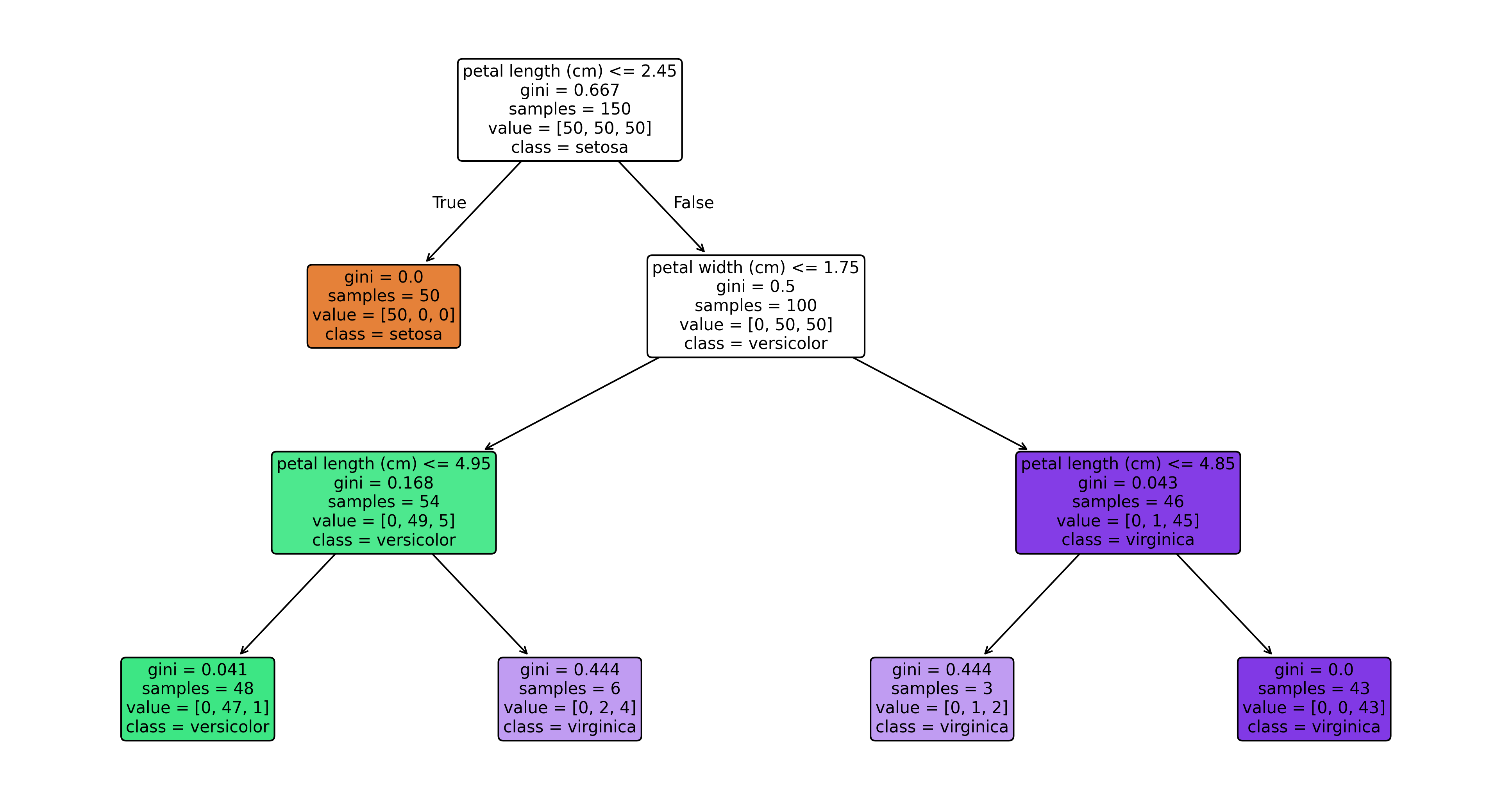
Every one of these threshold questions, in feature space, is a straight cut parallel to one of the axes: petal length < 2.45 slices the plane vertically, petal width < 1.75 slices it horizontally. Stack several of these axis-aligned cuts and the tree ends up carving the whole space into a grid of rectangles, each rectangle a leaf, each leaf's color the majority class of the training points that landed inside it.
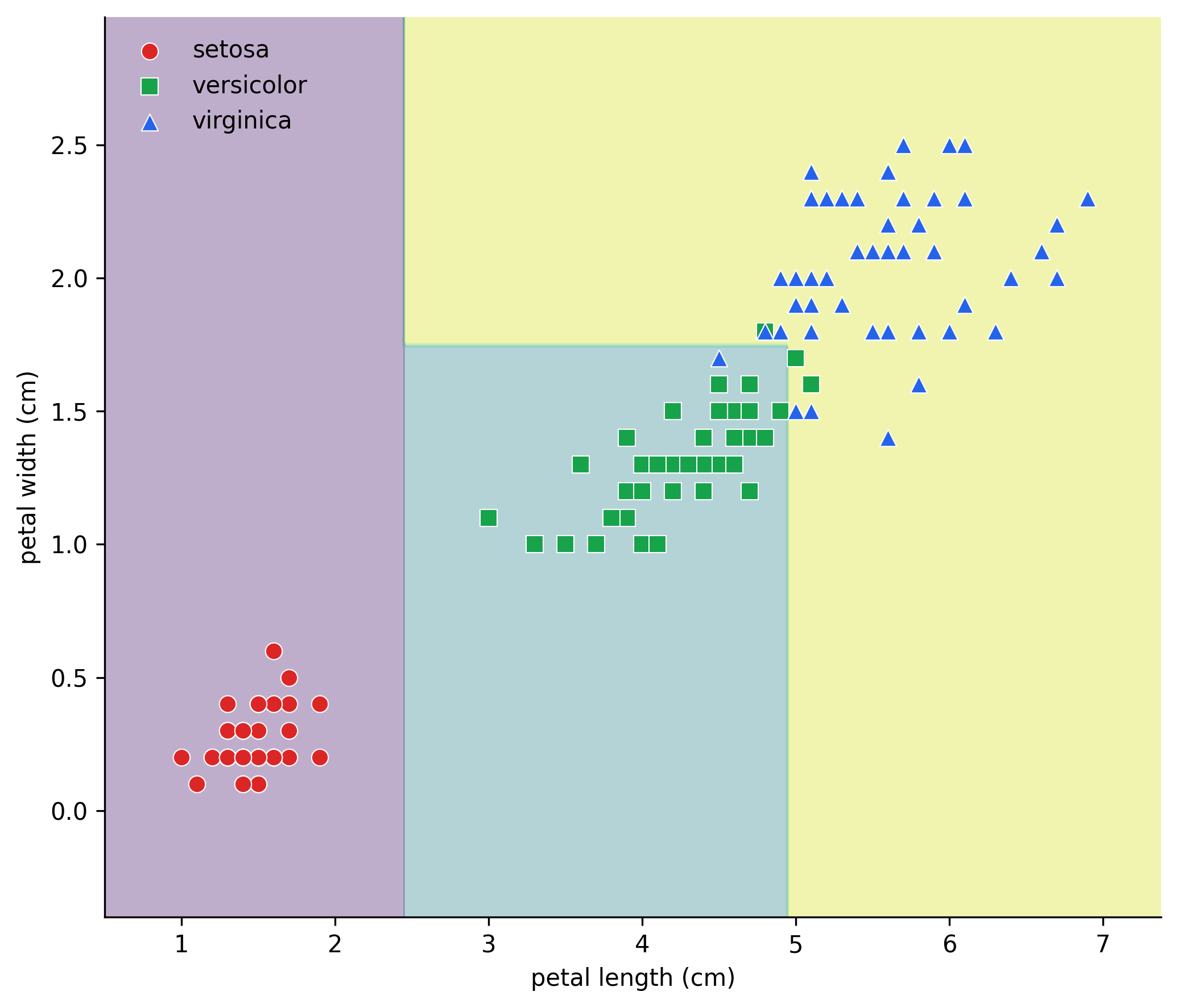
That's the geometric signature of a decision tree, worth contrasting with SVM's tilted straight line or KNN's locally-warped boundary: a decision tree's boundary is always a set of axis-aligned rectangles, because every single split can only ever cut along one feature at a time.
The actual fitted tree behind that picture, for reference on the terminology below:
6. Pseudocode
Stripped of any specific dataset, building a decision tree is a recursive procedure:
function build_tree(data):
    if all rows in data have the same label:
        return a leaf predicting that label

    question = pick the best feature (and threshold, if numeric) to split on
    left_data, right_data = split data using question

    left_branch = build_tree(left_data)
    right_branch = build_tree(right_data)
    return a decision node with (question, left_branch, right_branch)
Every worked example above followed exactly this shape by hand. The one line doing all the real work, pick the best feature to split on, is the part hand-waved through so far, and it's the entire subject of the next post.
7. Terminology
A quick reference for the vocabulary used throughout this series:
- Root node — the very first question, sitting at the top, applied to the entire dataset.
- Decision node (internal node) — any node that still asks a further question.
- Leaf node — a node with no further questions, holding a final prediction.
- Splitting — dividing a node's rows into child nodes based on a question.
- Pruning — the reverse of splitting: removing branches after the fact to fight overfitting.
- Parent / child — a node that splits is the parent of the two (or more) nodes it splits into.
8. Unanswered Questions
Building a tree by eyeballing a six-row table is easy; a real algorithm needs precise answers to two questions this post has deliberately left open:
- Which feature should a node split on, and, for numeric features, at what threshold? Some splits are far more useful than others,
occupationcleanly separated the Play Store example while a less-informative column wouldn't have. That "usefulness" needs a number attached to it. - When should splitting stop? A tree that keeps splitting until every leaf has exactly one row will fit the training data perfectly and generalize terribly.
Both are covered next, once entropy, information gain, and Gini impurity are introduced.
9. Advantages and Disadvantages
Advantages:
- Easy to interpret and explain, the tree can literally be drawn and read like a flowchart, no coefficients to squint at.
- Requires little data preparation: no feature scaling or standardization needed, since splits only ever compare a feature to a threshold, not to each other.
- Naturally handles both numeric and categorical features, and both classification and regression, without changing the core algorithm.
Disadvantages:
- Prone to overfitting: an unconstrained tree can memorize the training set by splitting all the way down to single-row leaves.
- Unstable: small changes in the training data can produce a noticeably different tree, since an early split near the root reshapes everything beneath it.
- Its axis-aligned boundaries are a poor geometric fit for data that's naturally separated by a diagonal or curved boundary, needing many small steps to approximate what a single line could do.
10. CART
The specific algorithm this series builds toward is called CART, Classification And Regression Trees. The name signals the two things covered later: the same splitting idea handles classification (predicting a category, as in every example above) and regression (predicting a number) alike, just with a different criterion for what makes a split "good." That criterion, and the fix for the overfitting problem above, is where entropy, information gain, and Gini impurity come in.