Ch.36: The Kernel Trick, In Code

Ch.35 built the geometric case for the kernel trick with two hand-picked examples: a 1D line lifted to 2D by squaring, and concentric circles lifted to 3D by $z = e^{-(x^2+y^2)}$. Both were true, and both dodged the actual question, in real code, how do you get that lift without manually inventing a formula for every dataset? This post runs the demo for real: an actual dataset, an actual failing SVM, an actual fix, and the sklearn keyword that makes the fix redundant.

1. A Linear SVM Fails on Circles

sklearn.datasets.make_circles generates exactly the shape Ch.35 described by hand: one class in a ring, the other clustered inside it. Fit a plain linear SVM on the raw two features and score it:

from sklearn.datasets import make_circles
from sklearn.svm import SVC
 
X, y = make_circles(n_samples=200, noise=0.06, factor=0.4, random_state=7)
 
linear_clf = SVC(kernel="linear").fit(X, y)
linear_clf.score(X, y)

0.59

59%, barely better than guessing. A straight line has no way to wall off a disc from the ring around it, exactly the limitation Ch.35 argued from geometry alone. Here it shows up as a number.

2. Fixing It by Hand

Ch.35's transform was $e^{-(x^2+y^2)}$; a simpler one works just as well here: $z = x_1^2 + x_2^2$, literally squared distance from the origin. Bolt it on as a third column and fit a linear SVM in 3D:

import numpy as np
 
z = X[:, 0] ** 2 + X[:, 1] ** 2
X3 = np.column_stack([X, z])
 
manual_clf = SVC(kernel="linear").fit(X3, y)
manual_clf.score(X3, y)

1.0

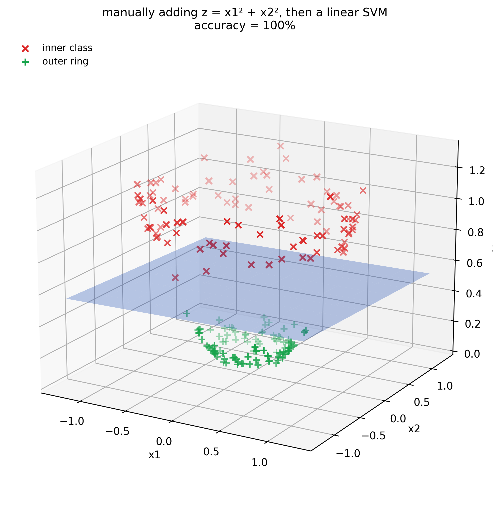
Perfect separation, same idea as Ch.35's picture, now backed by a classifier that actually scores 100%. The inner cluster sits close to the origin, so its $z$ stays small; the outer ring sits farther out, so its $z$ is large. One new coordinate, and a plane does the rest.

3. The Catch With Doing It by Hand

This worked because the shape of the data was known in advance, a ring around a core all but announces "use distance from the center." Real datasets don't come with that label. With more than two input features, there's no single obvious formula to reach for, and the space of candidate transforms, every pairwise product, every square, every cross-term, grows fast. Trying them one at a time and refitting each time doesn't scale past toy examples.

4. Skipping the Feature Entirely

This is where SVC's kernel argument earns its keep. Fit the same circles data again, still just the original two columns, no manually built $z$, but with kernel="rbf" instead of "linear":

rbf_clf = SVC(kernel="rbf", gamma="scale").fit(X, y)
rbf_clf.score(X, y)

1.0

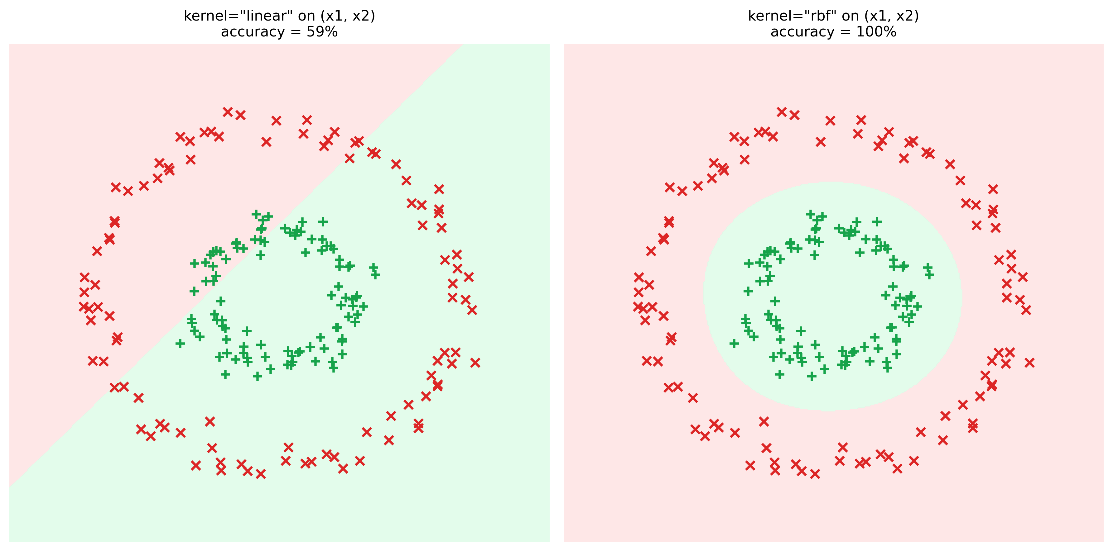
100% accuracy, and the decision boundary on the right is a circle, curved the way a straight line never could be, despite SVC never seeing a third feature. That's the trick: the RBF kernel produces the effect of lifting into a higher-dimensional space (in fact an infinite-dimensional one) without ever constructing a point in it. The actual mechanism, how a kernel function computes what's needed without visiting that space, is the math saved for the next post. What today's code confirms is that the effect is real and it's one argument away, not a manual feature-engineering project.

5. More Kernel Isn't Automatically Better

SVC ships a few kernel choices beyond rbf, including poly, whose flexibility is set directly by a degree argument. It's tempting to assume higher degree means a better fit, so it's worth checking that assumption on a harder dataset (make_moons, two interleaving crescents) with a held-out test split:

from sklearn.datasets import make_moons
from sklearn.model_selection import train_test_split
 
Xm, ym = make_moons(n_samples=120, noise=0.35, random_state=42)
Xm_train, Xm_test, ym_train, ym_test = train_test_split(Xm, ym, test_size=0.5, random_state=0)
 
for degree in [1, 3, 6, 10]:
    clf = SVC(kernel="poly", degree=degree, coef0=1, C=1).fit(Xm_train, ym_train)
    print(degree, clf.score(Xm_train, ym_train), clf.score(Xm_test, ym_test))

1   0.867  0.833
3   0.933  0.867
6   0.983  0.850
10  0.983  0.833

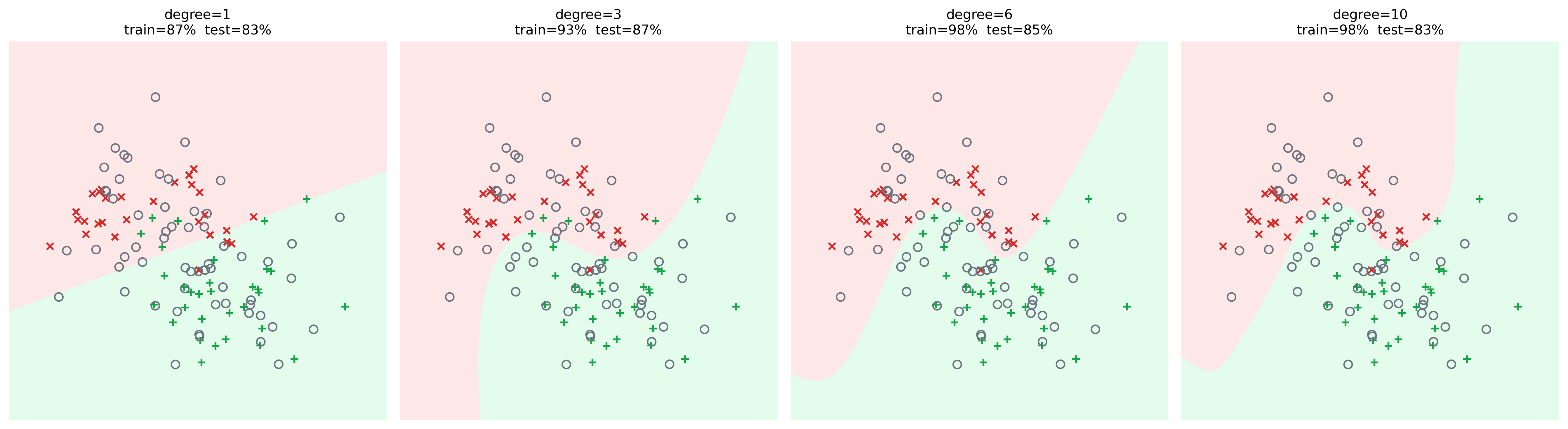
Training accuracy climbs the whole way, degree 10 fits the training points better than degree 1 ever could. Test accuracy doesn't: it peaks at degree 3 and drops back down by degree 10, and the boundary plots show why, at high degree the curve stops tracking the crescent shape and starts bending around individual points instead. A higher-degree kernel is a more flexible model, and like any flexible model it can memorize training data instead of learning the pattern in it. Picking a kernel and a degree is a bias-variance tradeoff (Ch.12) like any other, not a dial that only helps when turned up.