Ch.35: The Kernel Trick, Geometrically

By Ayush Arora•2026-08-30•5 min read

Inspired by: YouTube

Every SVM post so far, the intuition, hard margin's math, soft margin and hinge loss, has quietly assumed a straight line (or hyperplane) is the right shape to look for. Soft margin tolerates points that stray onto the wrong side of that line, but it's still hunting for a line. Some datasets don't have one to find, no matter how much slack is allowed. The kernel trick is how SVM handles those cases, and this post builds the intuition for it with two worked examples, entirely geometric, no kernel formula derived yet.

1. A 1D Dataset With No Separating Point

Start about as simple as classification gets: points on a single number line, each labeled red or green. Arrange them so the reds sit on both outer ends and the greens sit in the middle, red, green, red, left to right.

No single threshold value $t$ works here. Pick $t$ far enough right to catch the left red cluster, and every green point plus the right red cluster ends up on the same side, misclassified. Pick $t$ anywhere else and it's no better, there is no point on this line with reds on one side and greens on the other. In 1D, the "decision boundary" is just a threshold, a single dot on the line, and this data has no valid one.

2. Lifting It to 2D by Squaring

Take every point's value $x$ and compute a new coordinate $z = x^2$ , then plot $(x, z)$ instead of just $x$ . The red points, being further from zero, land at large $z$ values. The green points, clustered near zero, land at small $z$ values. Squaring turned "how far from the center" into an explicit coordinate.

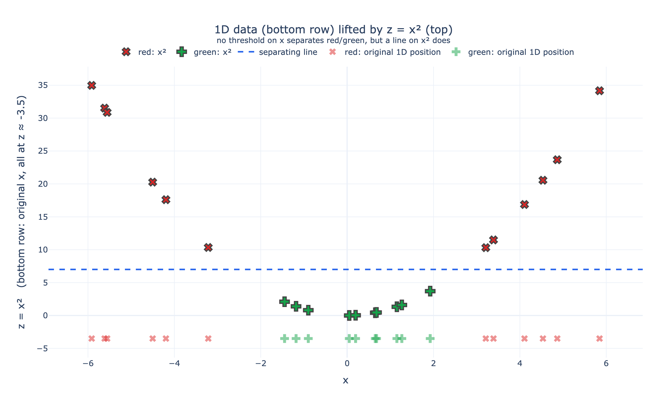
A 2D scatter plot. The bottom row shows the original 1D data along the x-axis, faded red x's on both outer ends and faded green plus signs in the middle, all sitting at the same low z value. Above it, the same points are plotted at z equals x squared: the red x's now sit high up since they were far from zero, the green plus signs sit low near z=0 since they were close to zero, and a horizontal blue dashed line cleanly separates the red points above it from the green points below it.

In this lifted 2D space, a plain horizontal line separates the classes perfectly, everything above it is red, everything below is green. That line didn't exist in the original 1D view, because there was no such line to draw, there's only one dimension in which to draw it. Adding the $z = x^2$ dimension didn't add information, it's fully determined by $x$ , but it rearranged the points into a space where a linear separator exists.

3. A Harder Case: Concentric Circles

The 1D example is deliberately easy to fix, one specific transform matches its exact structure. A tougher, genuinely 2D case: green points scattered in a ring, red points clustered inside that ring's hole. Every straight line drawn across this plane cuts through both colors, a circle's inside and outside can't be split by anything straight, that's what makes it a circle.

4. Lifting It to 3D

The same idea generalizes: add a third coordinate built from the existing two, $z = e^{-(x^2+y^2)}$ , a bump function that's tallest at the origin and decays outward. Since the red cluster sits near the origin, its points map to large $z$ . Since the green ring sits farther out, its points map to small $z$ , closer to $0$ .

A 3D scatter plot. Red x markers, originally a tight cluster near the center of the xy plane, are lifted high up along the z axis by the transform z equals e to the negative x squared plus y squared. Green plus markers, originally forming a ring around that cluster, stay low near z=0 since they are farther from the origin. A translucent blue horizontal plane sits between the two groups, with all red points above it and all green points below it.

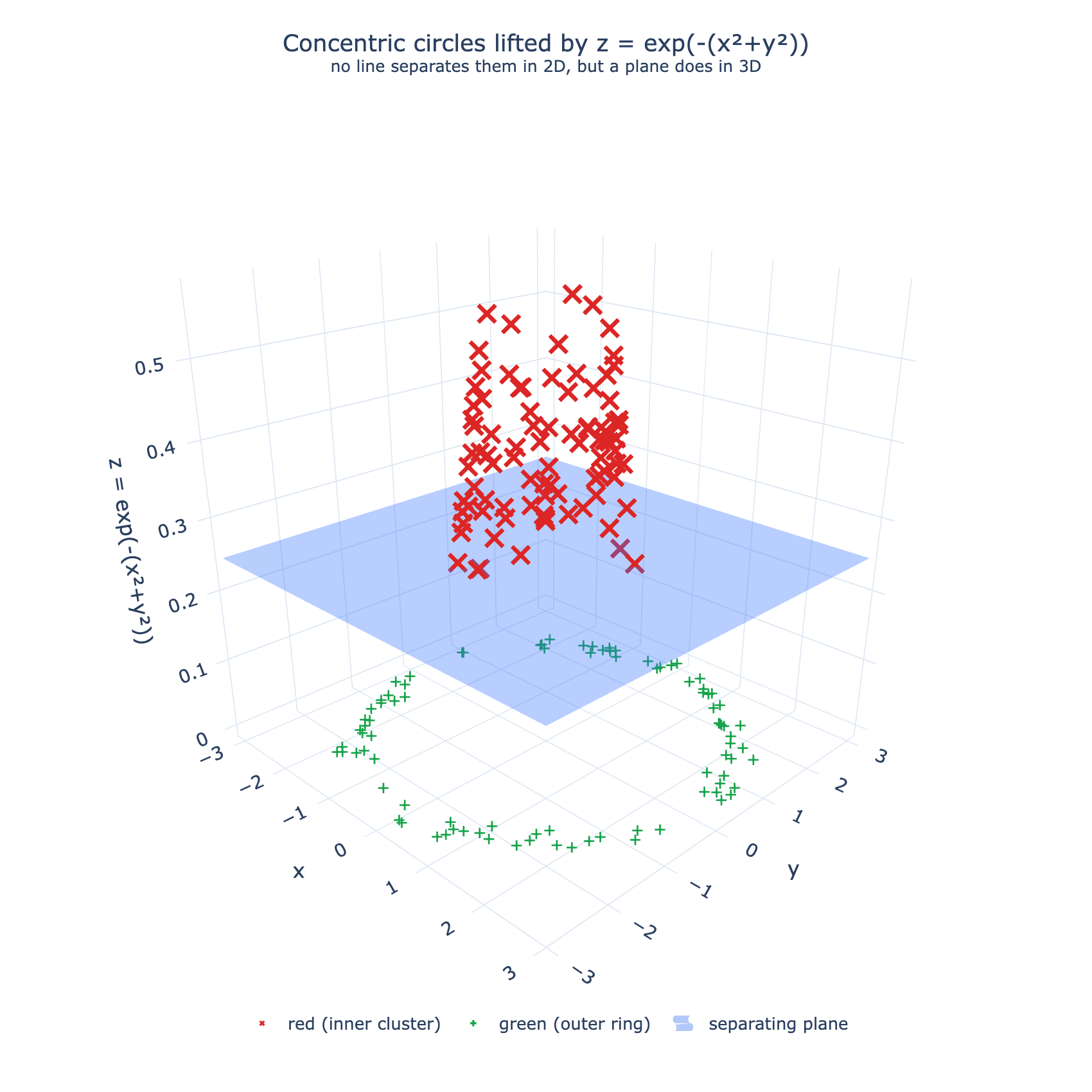
Plotted in 3D, with $z$ as a genuine third axis, a flat horizontal plane slices cleanly between the two classes: red above it, green below. Exactly the same move as the 1D case, one dimension short of separable, add a dimension built from a function of the existing coordinates, and a linear separator (a plane instead of a line, but still linear) appears where none existed before.

5. The General Pattern, and Where the "Trick" Comes In

Both examples follow the same recipe: take data that isn't linearly separable in its original space, apply some function $\phi$ that maps each point into a higher-dimensional space, and find that the images $\phi(x)$ are linearly separable there, even though the originals weren't. That mapping function $\phi$ is called a kernel, and three commonly used ones (deferred to a future post for their actual formulas) are the polynomial kernel, the sigmoid kernel, and the RBF (radial basis function) kernel, the last of which is exactly the family the $e^{-(x^2+y^2)}$ example above belongs to.

The "trick" part of "kernel trick" isn't in this post yet, it refers to something computational: explicitly transforming every point into a high-dimensional space and running SVM there would get expensive fast, especially since some useful kernels correspond to infinite-dimensional spaces. The actual trick is a way to get the effect of that transformation, the linear separator it makes possible, without ever computing $\phi(x)$ directly. That's the math saved for the next post; what should be solid from this one is why a transformation like this helps at all, illustrated concretely rather than asserted.

View all chapters in Machine Learning Algorithms →