Ch.33: The Math Behind Hard Margin SVM

Inspired by: YouTube

Last post left SVM at an intuitive level: among every line that separates the classes correctly, pick the one with the widest margin. That's a geometric idea, not yet something a computer can solve. This post turns it into an actual optimization problem, an objective and a set of constraints, entirely for the case where the data separates cleanly: hard margin SVM.

1. The Hyperplane and Its Two Supporting Planes

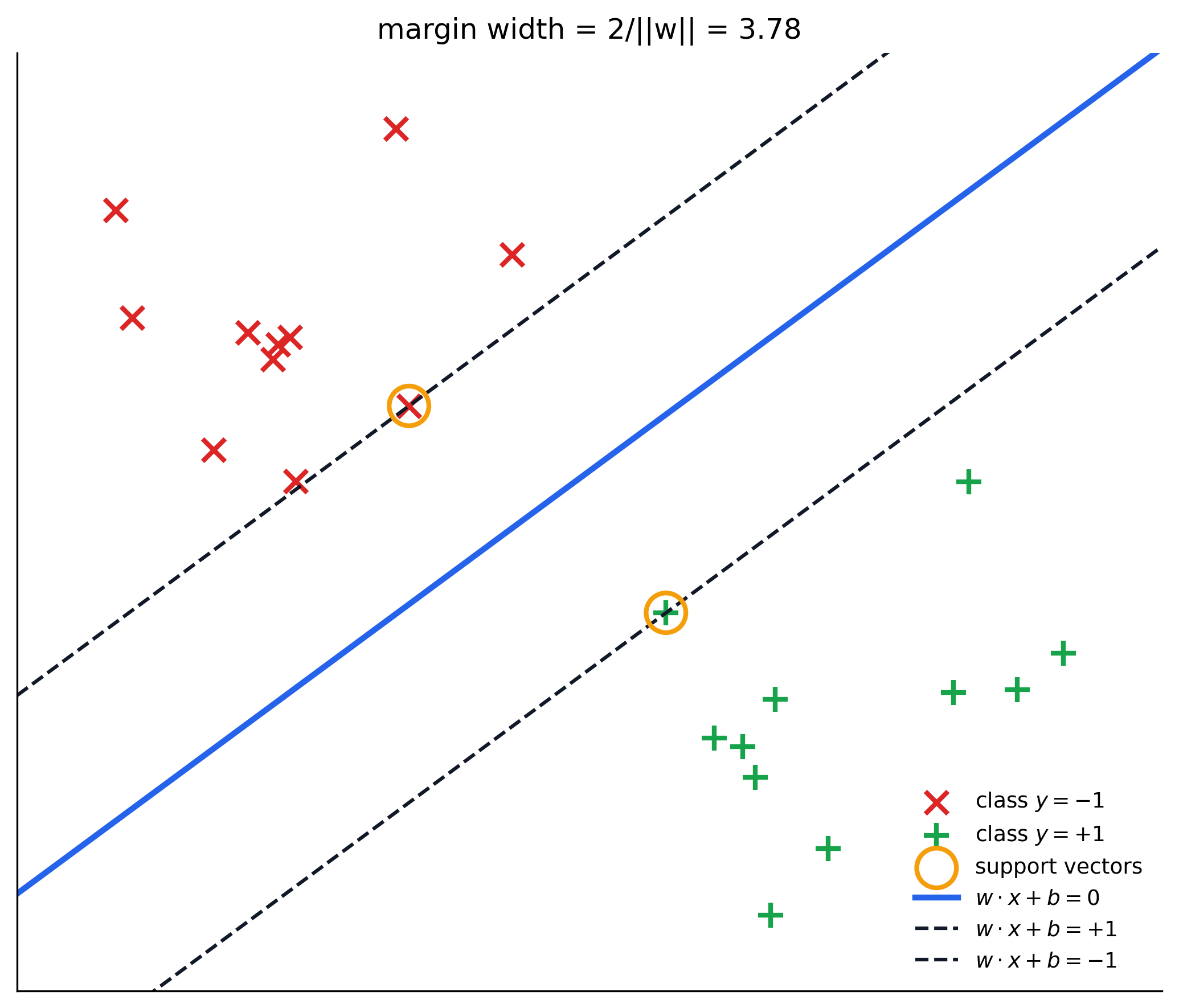
A linear decision boundary is written $w \cdot x + b = 0$, where $w$ is a weight vector and $b$ a bias, exactly like logistic regression's $z = w^Tx + b$. Points aren't just classified by which side of this line they fall on, they're pushed further: instead of stopping at $w \cdot x + b = 0$, define two more hyperplanes, parallel to it and shifted to just touch the nearest point of each class:

$w \cdot x + b = +1 \quad \text{(touches the nearest positive point)}$ $w \cdot x + b = -1 \quad \text{(touches the nearest negative point)}$

Every training point must sit on the correct side of its plane: positive-class points need $w \cdot x + b \geq 1$, negative-class points need $w \cdot x + b \leq -1$. Nothing is allowed inside the strip between the two planes, that strip is exactly the margin.

2. One Constraint Instead of Two

Labeling the classes $y = +1$ and $y = -1$ (not $0/1$, specifically so this trick works) turns the two separate conditions into a single inequality. Multiply both sides of each condition by its own label:

• Positive class: $y = +1$, and $w \cdot x + b \geq 1$, so $y(w \cdot x + b) \geq 1$.
• Negative class: $y = -1$, and $w \cdot x + b \leq -1$, multiplying by $-1$ flips the inequality: $y(w \cdot x + b) \geq 1$.

Both classes collapse into the same rule:

$y_i(w \cdot x_i + b) \geq 1 \quad \text{for every training point } i$

That's the constraint hard margin SVM has to satisfy for every single point, no exceptions. It's called "hard" precisely because of that: not one point is allowed to violate it, which only makes sense when the classes are actually linearly separable.

3. Margin Width, from the Distance Formula

The margin is the distance between the two supporting planes $w \cdot x + b = 1$ and $w \cdot x + b = -1$. The distance from a point $x_0$ to a plane $w \cdot x + b = c$ is the standard point-to-hyperplane distance:

$\text{distance} = \frac{|w \cdot x_0 + b - c|}{\|w\|}$

Take any point $x_1$ lying exactly on the positive plane, so $w \cdot x_1 + b = 1$. Its distance to the negative plane ($c = -1$) is:

$d = \frac{|w \cdot x_1 + b - (-1)|}{\|w\|} = \frac{|1 + 1|}{\|w\|} = \frac{2}{\|w\|}$

The margin width comes out to a strikingly simple expression: $d = \dfrac{2}{\|w\|}$. Wider margin means smaller $\|w\|$, and vice versa, the two are directly linked through this one formula.

4. From "Maximize the Margin" to a Solvable Problem

The goal is to maximize $d = 2/\|w\|$. Three standard rewrites turn that into the form actually handed to an optimizer:

1. Maximizing $2/\|w\|$ is the same as minimizing $\|w\|$, since $\|w\|$ sits in the denominator, shrink it and the margin grows.
2. Minimizing $\|w\|$ is the same as minimizing $\dfrac{1}{2}\|w\|^2$. Squaring removes the square root buried inside the norm, and dropping the square root makes the objective smooth and differentiable everywhere, which matters once calculus-based solvers take over. The constant $\frac{1}{2}$ is there purely to cancel a factor of $2$ that shows up when differentiating the square term later; it doesn't change which $w$ is optimal.
3. The constraints from Section 2 come along unchanged.

Putting it together, hard margin SVM is exactly this optimization problem:

$\min_{w, b} \frac{1}{2}\|w\|^2 \quad \text{subject to} \quad y_i(w \cdot x_i + b) \geq 1 \ \ \forall i$

A quadratic objective with linear inequality constraints is a convex quadratic program, a well-studied class of problem with a unique global minimum and no risk of getting stuck in a local one. That's what a solver like scikit-learn's SVC is actually solving under the hood; the Lagrangian-duality machinery used to solve it is its own topic, saved for when it's actually needed.

5. Why "Hard" Margin Specifically

Every step above leaned on one assumption: that some $w, b$ exists which satisfies $y_i(w \cdot x_i + b) \geq 1$ for all points simultaneously, in other words, that the data is perfectly linearly separable. If even one outlier sits on the wrong side, that constraint set has no solution at all, and this formulation simply fails to run, not just runs poorly.

That's the gap flagged at the end of the previous post: real data is rarely this clean. The fix is soft margin SVM, which relaxes the constraint to tolerate some points crossing the line, at a controlled cost. That relaxation, and the slack variable that makes it precise, is the next post.