
Ch.26: Precision, Recall, and F1 Score
Inspired by: YouTube
Ch.25 ended with accuracy failing badly on an imbalanced dataset, a model that always says "not a terrorist" scores 99.9999% accuracy while being useless at its one job. This post covers the two metrics built to catch exactly that kind of failure: precision and recall.
1. When Accuracy Can't Break a Tie
Say two junior engineers each built a spam classifier, and the better one gets deployed. Both models' confusion matrices give the exact same accuracy, 80%. Accuracy alone can't tell them apart, so something else has to.
Looking closer, the two models differ in where their mistakes land. One has more false positives (real emails wrongly flagged as spam), the other has more false negatives (spam wrongly let into the inbox). Which mistake matters more here? A missed spam email is a mild annoyance, but a real email wrongly buried in spam, say, a job offer with a reply deadline, can cost something real. So the more dangerous error for this problem is the false positive, and the better model is whichever one commits fewer of them.
That comparison is exactly what precision measures.
2. Precision
In words: of everything the model predicted positive, what fraction was actually positive. A model with high precision is one that, when it says "spam," is usually right.
As a worked example: say the mail dataset has 1000 emails, 300 actually spam and 700 actually not. Both candidate models get 800 out of 1000 correct (80% accuracy), but split their 200 mistakes differently:
- Model A: FP = 50, FN = 150 → , so precision
- Model B: FP = 150, FN = 50 → , so precision
Model A has fewer false positives and the higher precision, against , so it's the one to deploy, exactly matching the "false positives are the dangerous mistake here" judgment from Section 1.
3. Recall
Now flip the scenario: two models screening chest X-rays for cancer, again tied at the same accuracy. Here the dangerous mistake runs the other way. A false positive means telling a healthy patient they might have cancer, unpleasant, but resolved with follow-up tests. A false negative means telling a patient with real cancer that they're fine, a missed diagnosis that can cost a life. This time the more dangerous error is the false negative, and the model to prefer is whichever one commits fewer of them.
That's recall:
In words: of everything that's actually positive, what fraction did the model correctly catch. A model with high recall rarely lets a real positive slip through.
Same style of worked example: 1000 patients, 200 actually have cancer, 800 don't, both models at 90% accuracy (900 correct, 100 mistakes), split differently:
- Model A: FP = 80, FN = 20 → , so recall
- Model B: FP = 20, FN = 80 → , so recall
Model A misses fewer real cancer cases and has the higher recall, against , so it's the model to deploy here.
4. The General Rule, and Where It Breaks Down
Putting Sections 2 and 3 together: if a Type I error (false positive) is the more dangerous mistake for a given problem, pick the model with higher precision. If a Type II error (false negative) is more dangerous, pick the model with higher recall.
But this rule needs one input the model can't give you: knowing, for the problem at hand, which error type is actually worse. Sometimes that's not obvious. Take a classifier that looks at a photo and predicts cat or dog: is mislabeling a cat as a dog worse, or mislabeling a dog as a cat? There's no clear answer, both errors are just "got it wrong" with no asymmetric real-world cost attached. In cases like this, precision and recall have to be weighed together rather than picking one, and (as later posts in this series cover) the two trade off against each other, pushing one up tends to pull the other down.
5. F1 Score: Combining the Two
When both matter and there's no reason to strictly prefer one, a single combined number is convenient: the F1 score, the harmonic mean of precision and recall.
The choice of harmonic mean over a plain arithmetic mean is deliberate: a harmonic mean always sits closer to the smaller of its two inputs, so a model that's weak in either precision or recall gets penalized, it can't hide a bad score behind one strong number.
Compare arithmetic and harmonic mean on an extreme case: precision , recall . Arithmetic mean is , a number that suggests a decent model. Harmonic mean is , which correctly reflects that a model with 2% precision is close to useless despite its perfect recall.
A subtler case makes the same point without an extreme: Model A has precision , recall . Model B has precision , recall . Both have an arithmetic mean of exactly , a tie. But their F1 scores:
F1 correctly ranks Model A higher, against , because it penalizes Model B for its weaker precision even though B's perfect recall pulled the plain average even. That's the entire reason F1 uses the harmonic mean instead of the arithmetic one.
6. Computing All Three for Real
Running precision_score, recall_score, and f1_score on the same heart disease models from Ch.25, following the source notebook:
from sklearn.metrics import precision_score, recall_score, f1_score

print("Precision:", precision_score(y_test, y_pred1))
print("Recall:", recall_score(y_test, y_pred1))
print("F1:", f1_score(y_test, y_pred1))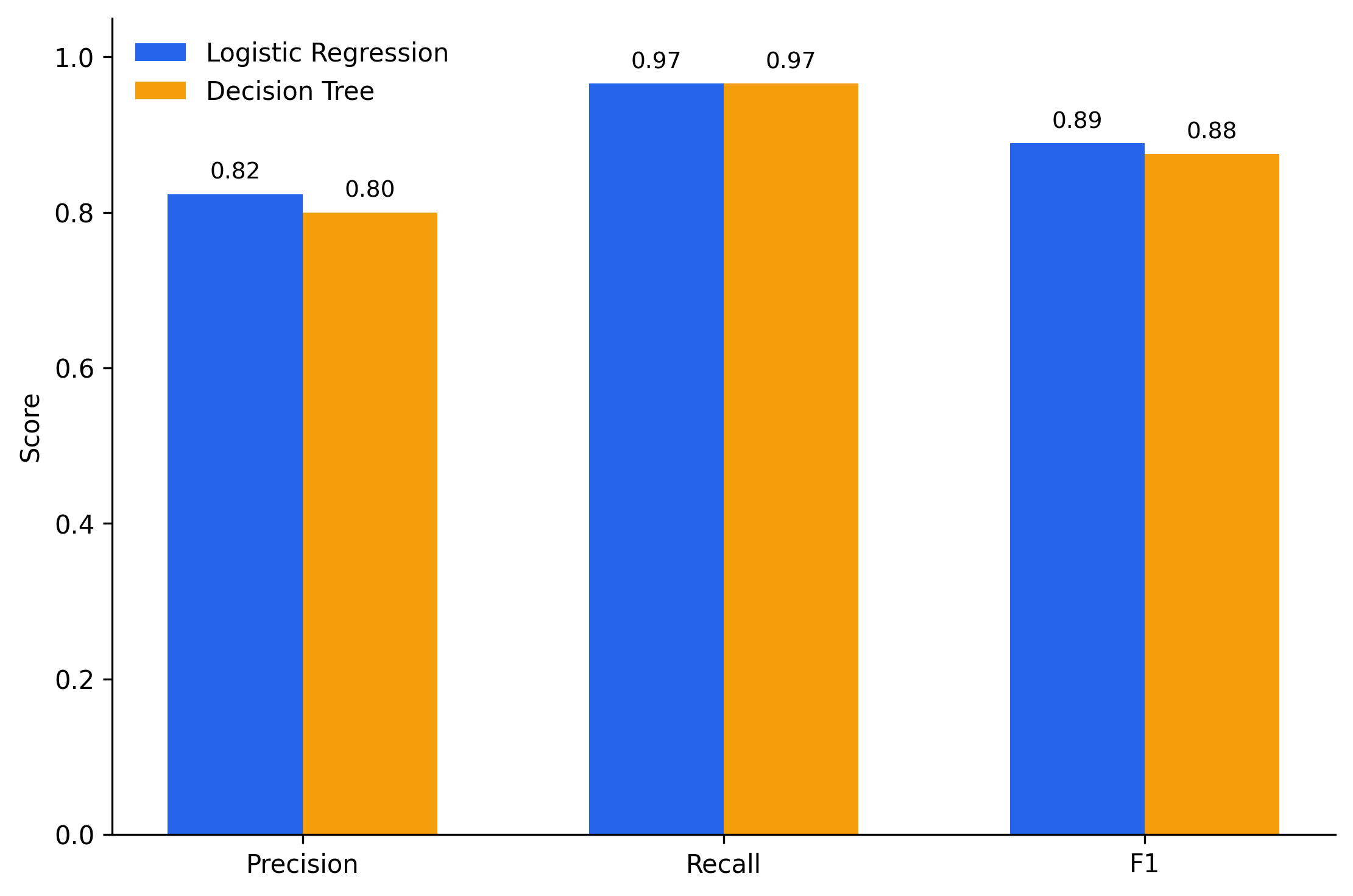
Both models catch almost every real case of heart disease (recall for both), but Logistic Regression has the edge on precision (0.82 against 0.80), giving it the slightly higher F1 (0.89 against 0.88), consistent with it being the better model on this dataset in Ch.25 too.
7. Precision and Recall for More Than Two Classes
Binary classification usually has a clear "positive" class to focus on, spam vs. not spam, cancer vs. not, so precision and recall are reported for that one class. With more than two classes, there's no single class to elevate above the others, so precision and recall get computed once per class, each one asking "treat this class as positive, everything else as negative" and applying the same formulas as before.
As a worked illustration, take a 3-class dog/cat/rabbit classifier evaluated on 100 labeled photos, where rabbits are rare in the dataset (only 5 out of 100):
| Actual \ Predicted | Dog | Cat | Rabbit | Actual total |
|---|---|---|---|---|
| Dog | 40 | 8 | 2 | 50 |
| Cat | 5 | 40 | 0 | 45 |
| Rabbit | 1 | 3 | 1 | 5 |
| Predicted total | 46 | 51 | 3 | 100 |
Precision and recall computed per class:
- Dog: precision , recall
- Cat: precision , recall
- Rabbit: precision , recall
Three numbers per metric is often more detail than needed, so they get collapsed into one of two combined scores:
- Macro average: the plain mean across classes. Macro precision .
- Weighted average: the mean weighted by each class's support (how many actual instances it has). Weighted precision .
The gap between them, versus , is the whole point of having both. Rabbit is both rare and badly predicted (precision ), and the weighted average, dominated by the much larger Dog and Cat classes, barely notices it. The macro average weighs Rabbit's poor score equally with the other two, so it drags the overall number down and surfaces the problem. The convention: use macro average when classes are roughly balanced, and weighted average when they're imbalanced, but as this example shows, weighted average can specifically hide how badly a rare class is being handled, worth keeping in mind rather than following blindly.
8. Multi-Class, For Real
The same per-class-then-combine logic on a real dataset, Iris, following the multi-class notebook:
from sklearn.metrics import precision_score, recall_score

precision_score(y_test, y_pred1, average=None)     # per-class
precision_score(y_test, y_pred1, average="macro")
precision_score(y_test, y_pred1, average="weighted")
Running this on a held-out Iris test split gives per-class precision of [1.0, 1.0, 0.857] and per-class recall of [1.0, 0.923, 1.0] across the three species, a macro precision of 0.952, and a weighted precision of 0.971.
sklearn also bundles all of this into one call, classification_report, run here on a 10-class handwritten-digit dataset (the source notebook uses Kaggle's full MNIST train.csv; the results below use sklearn's bundled load_digits, the same style of problem at a size that runs anywhere):
from sklearn.metrics import classification_report
print(classification_report(y_test, y_pred))
precision recall f1-score support
0 1.00 0.97 0.98 32
1 0.95 0.95 0.95 44
2 1.00 1.00 1.00 31
3 0.97 0.92 0.94 36
4 0.94 0.89 0.91 35
5 0.98 0.95 0.96 43
6 1.00 0.94 0.97 35
7 0.97 0.97 0.97 40
8 0.81 0.97 0.89 36
9 0.86 0.89 0.88 28
accuracy 0.95 360
macro avg 0.95 0.95 0.95 360
weighted avg 0.95 0.95 0.95 360
One table, every class's precision, recall, and F1, plus both combined averages and overall accuracy, exactly the numbers Sections 7 and 8 built up by hand, computed in a single line.
9. What's Next
Section 4 left an open thread: precision and recall trade off against each other, pushing one up tends to pull the other down. That trade-off, and how to navigate it deliberately instead of by accident, is next.