Ch.18: Why Lasso Zeroes Out Coefficients (And Ridge Never Does)

Inspired by: YouTube

Ch.17 established the difference empirically: Ridge coefficients shrink toward zero but never reach it, Lasso coefficients can land on exactly zero. That's a famous machine learning interview question, ask why, and the honest answer needs the actual closed-form math, not just the shrink-vs-zero observation. This post derives it.

1. Setting Up the Same Way as Ridge

Start the same way the video does. The loss is

$L = \sum_{i=1}^n (y_i - \hat y_i)^2 + \lambda |m|$

Substituting $\hat y_i = mx_i + b$ and then $b = \bar y - m\bar x$ turns that into

$L = \sum_{i=1}^n (y_i - mx_i - \bar y + m\bar x)^2 + \lambda |m| = \sum_{i=1}^n \big[(y_i - \bar y) - m(x_i - \bar x)\big]^2 + \lambda |m|$

Ridge's version of this (Ch.14) replaced the last term with $\lambda m^2$, which is smooth everywhere and differentiates cleanly, giving $m = \dfrac{\sum (y_i - \bar y)(x_i - \bar x)}{\sum (x_i - \bar x)^2 + \lambda}$ directly. Lasso's $\lambda |m|$ is not differentiable at $m = 0$, an absolute value has a sharp corner there, so the single clean derivative doesn't exist. That corner is the entire reason this post needs three cases instead of one.

2. Three Cases Instead of One Derivative

Right before splitting into cases, the video makes one small algebra move for convenience: it writes the penalty as $2\lambda|m|$ instead of $\lambda|m|$. Nothing about the model changes, this is just relabeling the penalty's strength so that the factor of $2$ produced by differentiating the squared term cancels cleanly, instead of leaving a $\lambda/2$ sitting in every formula.

Case $m > 0$: here $|m| = m$, so $L = \sum\big[(y_i-\bar y) - m(x_i-\bar x)\big]^2 + 2\lambda m$, an ordinary smooth parabola. Differentiating with respect to $m$ and setting it to zero:

$\frac{dL}{dm} = -2\sum(x_i-\bar x)\big[(y_i-\bar y) - m(x_i-\bar x)\big] + 2\lambda = 0$

Dividing through by $2$ and solving for $m$:

$m = \frac{\sum(x_i-\bar x)(y_i-\bar y) - \lambda}{\sum(x_i-\bar x)^2}$

This is only a valid solution if it actually lands in $m > 0$, i.e. if $\sum(x_i-\bar x)(y_i-\bar y) > \lambda$.

Case $m < 0$: here $|m| = -m$, and setting the derivative to zero the same way:

$m = \frac{\sum(x_i-\bar x)(y_i-\bar y) + \lambda}{\sum(x_i-\bar x)^2}$

Valid only if this lands in $m < 0$, i.e. if $\sum(x_i-\bar x)(y_i-\bar y) < -\lambda$.

Case $m = 0$: at the corner itself, $|m|$ doesn't have a single derivative, it has a subgradient, every slope value between $-2\lambda$ and $2\lambda$ counts as valid at that one point. The minimum sits at $m=0$ whenever zero is among those valid slopes, which works out to exactly when neither of the two cases above was satisfiable, i.e. $\left|\sum(x_i-\bar x)(y_i-\bar y)\right| \le \lambda$.

To keep the three cases readable side by side, write $\text{num} = \sum(x_i-\bar x)(y_i-\bar y)$ and $\text{den} = \sum(x_i-\bar x)^2$, plain OLS's own numerator and denominator. Put together, this is the soft-thresholding formula:

$m^* = \begin{cases} \dfrac{\text{num} - \lambda}{\text{den}} & \text{num} > \lambda \quad (m > 0) \\[6pt] 0 & |\text{num}| \le \lambda \quad (m = 0) \\[6pt] \dfrac{\text{num} + \lambda}{\text{den}} & \text{num} < -\lambda \quad (m < 0) \end{cases}$

3. Why This Actually Reaches Zero and Ridge's Formula Never Does

Line up the two formulas directly:

$m_{\text{Ridge}} = \frac{\text{num}}{\text{den} + \lambda} \qquad\qquad m_{\text{Lasso}} = \frac{\text{num} \mp \lambda}{\text{den}}$

Ridge's $\lambda$ lives in the denominator. Growing $\lambda$ makes the denominator bigger, which makes the fraction smaller, but a nonzero numerator divided by any finite number is still nonzero. The only way Ridge's $m$ hits exactly zero is if the numerator itself was zero to begin with. That's the whole reason Ch.16's point 1 holds: shrinkage without ever quite arriving.

Lasso's $\lambda$ lives in the numerator, subtracted directly from it. Once $\lambda$ grows past $|\text{num}|$, the numerator would have to cross zero and flip sign, but the case split forbids that: the $\text{num} - \lambda > 0$ branch is only valid while it's positive, and the $\text{num} + \lambda < 0$ branch is only valid while it's negative. The moment neither branch's own condition holds anymore, the formula falls through to the third case and locks $m$ at exactly $0$, and it stays there for every larger $\lambda$ afterward, there's no branch left that would ever pull it back off zero. That's the algebraic reason feature selection is possible: the penalty competes directly against the numerator, and once it wins, it wins outright.

4. Verifying Against Scikit-Learn

sklearn.linear_model.Lasso doesn't use this post's exact loss, it minimizes $\frac{1}{2n}\text{RSS} + \alpha|w|$ rather than $\text{RSS} + 2\lambda|w|$, so its alpha and this derivation's $\lambda$ differ by a factor of $n$: $\lambda = n\alpha$. Accounting for that, the closed-form soft-threshold and Lasso.coef_ should match exactly:

import numpy as np
from sklearn.datasets import make_regression
from sklearn.linear_model import Lasso
 
X, y = make_regression(n_samples=100, n_features=1, n_informative=1, n_targets=1, noise=20, random_state=13)
x = X.ravel()
n = len(x)
 
xbar, ybar = x.mean(), y.mean()
num = np.sum((x - xbar) * (y - ybar))
den = np.sum((x - xbar) ** 2)
 
def soft_threshold_m(lam):
    if num > lam:
        return (num - lam) / den
    elif num < -lam:
        return (num + lam) / den
    return 0.0
 
for alpha in [0, 0.5, 1, 2, 5, 10, 50]:
    lam = n * alpha
    print(alpha, soft_threshold_m(lam), Lasso(alpha=alpha).fit(X, y).coef_[0])
# 0    27.8281  27.8281
# 0.5  27.2524  27.2524
# 1    26.6766  26.6766
# 2    25.5251  25.5251
# 5    22.0707  22.0707
# 10   16.3133  16.3133
# 50    0.0000   0.0000

Every value matches to four decimal places. The derivation also predicts exactly where the coefficient should hit zero: solving $\text{num} = \lambda = n\alpha$ for $\alpha$ gives $\alpha^* = \text{num}/n$, which computes to 24.17 for this dataset. Scanning Lasso's actual output near that boundary confirms it:

for alpha in [24.0, 24.16, 24.17, 24.2, 25]:
    print(alpha, Lasso(alpha=alpha).fit(X, y).coef_[0])
# 24.0   0.1927
# 24.16  0.0084
# 24.17  0.0
# 24.2   0.0
# 25     0.0

The coefficient is still (barely) nonzero at alpha=24.16 and has snapped to exactly 0.0 by alpha=24.17, right where the formula says it should.

5. Ridge and Lasso Side by Side

Plotting both coefficient paths on the same synthetic dataset makes the numerator-vs-denominator difference visible directly:

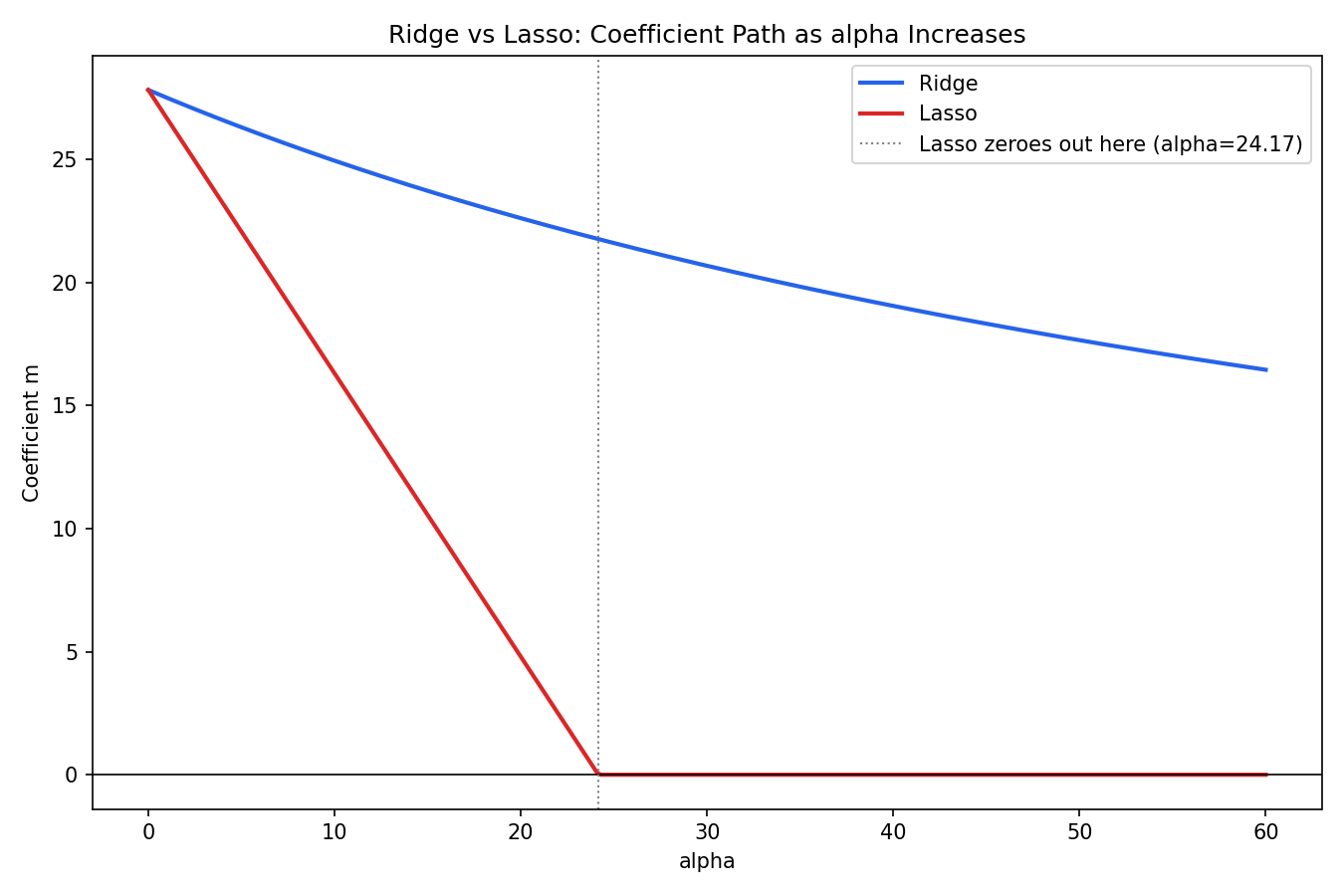
Both curves start at the exact same point, m≈27.83, because at alpha=0 both formulas collapse back to plain OLS. From there they diverge, and the shape of each curve is a direct fingerprint of where $\lambda$ sits in its formula.

Ridge's $m = \text{num}/(\text{den}+\lambda)$ has $\lambda$ in the denominator, so the curve is a hyperbola: growing $\lambda$ makes the denominator bigger, which shrinks the fraction, but a nonzero numerator divided by an ever-larger number only ever approaches zero, it never lands on it. That's why the blue curve keeps bending flatter without ever touching the x-axis, still sitting above 16 even at alpha=60.

Lasso's $m^* = (\text{num}-\lambda)/\text{den}$ has $\lambda$ in the numerator instead, with $\text{den}$ just a fixed constant out front. That makes it a straight line in $\lambda$ with slope $-1/\text{den}$, right up until the case split kicks in: once $\lambda$ passes num (here alpha=24.17), the formula switches to the third case and pins $m$ at exactly 0 for good. So the red line isn't a curve that happens to hit zero, it's a straight line that gets clipped the moment it would try to cross zero, which is exactly what the case-by-case derivation in section 2 predicts.

Same starting point, same-looking algebra, and the only structural difference, numerator versus denominator, is enough to turn one into a curve that never arrives and the other into a line that arrives and stops.

This derivation only covers the single-feature case, matching how the intuition is easiest to see. The general multi-feature version doesn't have as clean a closed form since the $|w_j|$ terms don't separate as neatly, and Scikit-Learn's actual Lasso solves it with coordinate descent instead. That from-scratch implementation is the next post.