
Ch.23: Discretization and Binarization: Turning Numbers into Categories
Inspired by: YouTube
So far in this feature engineering series, most of the work has gone one direction: taking messy categorical data and turning it into numbers a model can use. This post flips that around. Sometimes a numerical column actually works better once it's converted into categories. The two techniques for doing that are Discretization (also called Binning) and Binarization.
Why Turn Numbers Into Categories?
Picture a Google Play Store dataset with a "Number of Downloads" column. Some apps have a huge number of downloads, most have very few, and the raw numbers are scattered all over the place: some tiny, some in the millions. Instead of using the raw count, you could group it into buckets like "1M+ downloads", "100K+ downloads", "10K+ downloads", and so on.
That's exactly what discretization does. Grouping the raw numbers into a handful of buckets turned a messy, spread-out column into a clean categorical one, and made a real machine learning problem easier to work with. That's the motivation for this whole post: sometimes your numerical data has a better representation as categories.
What Is Discretization (Binning)?
Discretization is the process of transforming a continuous numerical column into a discrete one by creating a set of intervals, called bins, and sorting every value into whichever bin it falls into. It's also commonly called Binning. Think of a histogram: you're doing exactly the same thing a histogram does when it groups values into bars, except here the output is a new column you can actually use as a feature.
Binning gives you two concrete benefits:
- It handles outliers better. An extreme value at the far end of the data gets placed into the last bin along with other values in that same range. Once it's in a bin, it's treated exactly the same as its neighbors, so the model no longer sees it as a wild extreme value.
- It can improve the value spread. If most of your data is bunched up in one area, certain binning strategies can spread that bunched-up data out more evenly across bins.
Binning turns "this value is 47,382,910" into "this value is in the top bucket." The exact number stops mattering; only which group it belongs to does.
Three Categories of Binning
This post focuses on the three unsupervised techniques, plus a quick look at custom binning. Decision Tree binning uses the target column to pick cut points, which is a big enough topic to deserve its own dedicated post later.
Equal Width (Uniform) Binning
This is the simplest version, and it works exactly like drawing a histogram. You pick how many bins you want, and the column's range gets sliced into that many equal-width chunks:
bin_width = (max_value - min_value) / number_of_bins
Say a column ranges from 0 to 100 and you ask for 10 bins. Each bin is 10 units wide: 0-10, 10-20, 20-30, and so on up to 90-100. Every value gets sorted into whichever slice it falls in.
What it's good for: handling outliers. A value way out at the top of the range just lands in the last bin along with everything else near it, and gets treated like any other value in that bin.
What it doesn't do: change how the data is spread out. If most of your values were bunched up in the middle before binning, they're still bunched up into the same few middle bins after binning. The shape of the distribution stays the same; it's just chopped into discrete steps now.
Equal Frequency (Quantile) Binning
Here the goal flips: instead of making every bin the same width, you make every bin hold roughly the same number of rows. This is also called Quantile Binning, because the cut points come from percentiles.
Say you ask for 10 bins. The first bin runs from the minimum value up to the 10th percentile, so it holds about 10% of the data. The second bin runs from the 10th percentile to the 20th percentile, holding another 10%, and so on, all the way to the 100th percentile. The bins themselves can be very different widths: a bin covering a crowded part of the data might be narrow, while a bin covering a sparse stretch might be wide. What stays consistent is the count of rows in each one.
Quantile binning gives you two benefits at once:
- It handles outliers just as well as Equal Width binning.
- It also evens out the value spread, since by construction every bin ends up with a similar number of items.
Because of that second benefit, Quantile binning tends to get used more often than Equal Width, and it's the strategy scikit-learn reaches for by default.
K-Means Binning
This one is different: instead of slicing the range or the percentiles, it looks for natural groupings in the data using the K-Means clustering algorithm.
K-Means works like this:
- Randomly place a handful of "centroids" (cluster centers) somewhere among the data.
- Assign every point to whichever centroid is closest to it. Each centroid now "owns" a group of points.
- Move each centroid to the actual mean position of the points assigned to it.
- Repeat steps 2 and 3. Points get reassigned to whichever centroid is now closest, centroids shift again, and this continues until nothing changes anymore.
Once it settles, each centroid represents one bin, and every point belongs to the bin of its nearest centroid. The bin edges themselves fall at the midpoint between each pair of neighboring centroids.
Here's that process on a synthetic column with three natural clumps of values (150, 400, and 100 points respectively, with real gaps between them): three centroids are dropped in randomly, then K-Means reassigns points and slides the centroids to the mean of their group until nothing moves anymore.
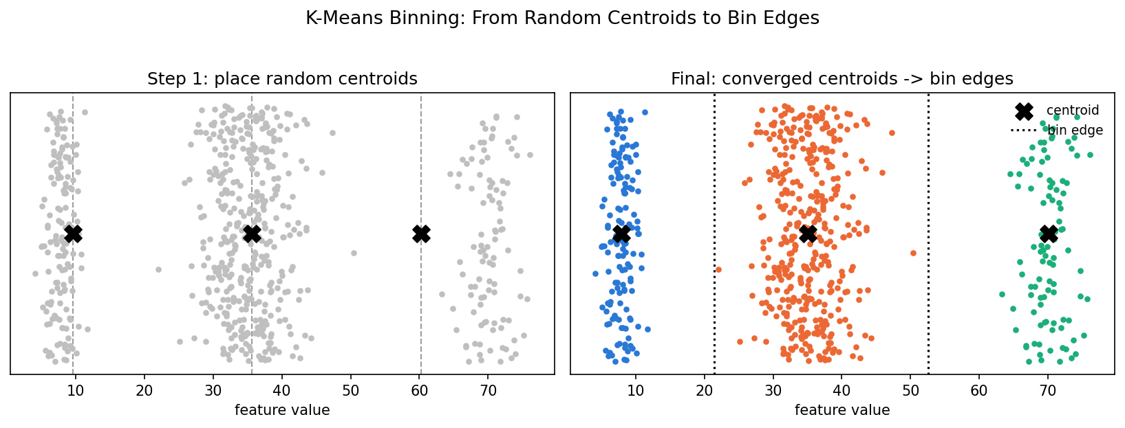
Notice where the final dotted bin-edge lines land: right in the empty gaps between clusters, not through the middle of any of them. That's the key difference from Equal Width or Quantile binning, which don't know anything about where the data actually clusters:
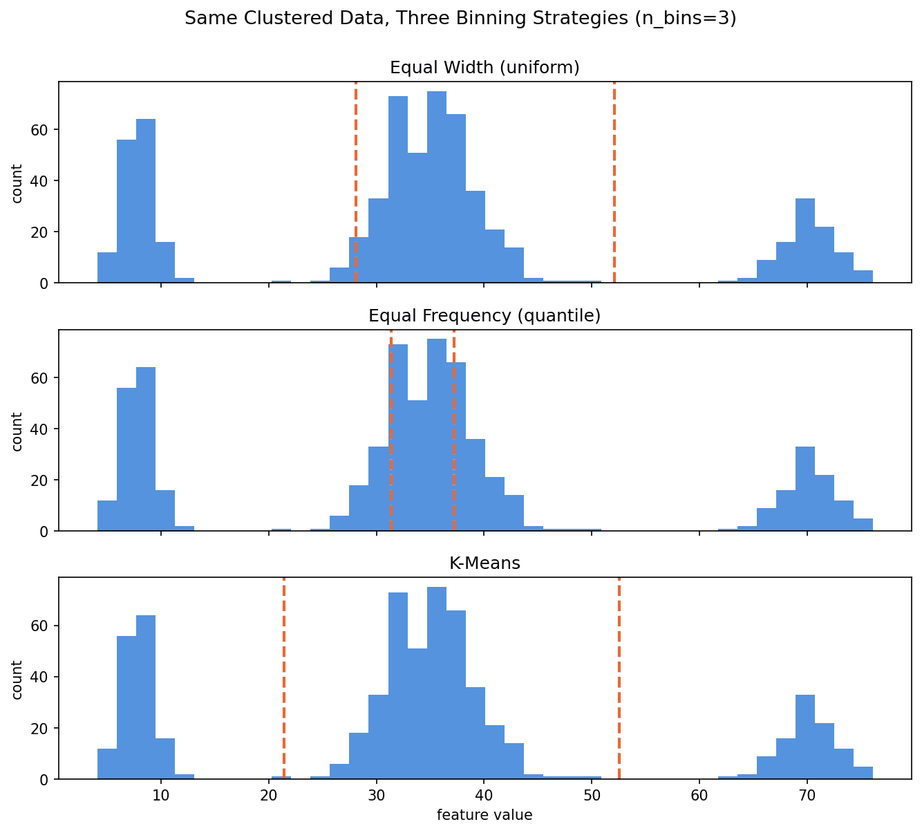
Equal Width slices a bin edge straight through the middle cluster because it only looks at min and max, it has no idea that a cluster boundary sits nearby. Quantile does a little better but still drops both of its edges inside that same middle cluster, since it's just chasing an equal row count per bin and that cluster happens to hold most of the data. K-Means is the only one of the three that actually looks at the shape of the data and lands its edges in the natural gaps, which is exactly why it's the strategy to reach for when a column looks clustered rather than smoothly spread out.
K-Means binning is most useful when your data naturally clumps into groups, with visible gaps between clusters rather than one smooth spread. If the data doesn't have that clustered shape, Equal Width or Quantile binning generally does a fine job on their own.
KBinsDiscretizer in scikit-learn
All three unsupervised strategies above are available through a single class: KBinsDiscretizer. You control it with three parameters:
| Parameter | What It Controls |
|---|---|
n_bins | How many bins to create |
strategy | 'uniform', 'quantile', or 'kmeans' |
encode | How the bin labels get output: 'ordinal' (a single integer column) or one-hot |
from sklearn.preprocessing import KBinsDiscretizer

kbin = KBinsDiscretizer(n_bins=10, encode='ordinal', strategy='quantile')
X_train_binned = kbin.fit_transform(X_train[['Age', 'Fare']])

X_train[['Age', 'Fare']].sample(5, random_state=42)
Age Fare
254 41.0 20.2125
278 7.0 29.1250
869 4.0 11.1333
539 22.0 49.5000
391 21.0 7.7958import pandas as pd
pd.DataFrame(X_train_binned, columns=['Age', 'Fare'], index=X_train.index).sample(5, random_state=42) Age Fare
254 7.0 5.0
278 0.0 7.0
869 0.0 3.0
539 3.0 7.0
391 2.0 1.0Same five rows, before and after. Age and Fare go from raw continuous values to a bin index between 0 and 9. Row 254, for instance, had an Age of 41.0, one of the older passengers in the training set, and it landed in bin 7, near the top end of the 10 age bins.
encode='ordinal' is the more common choice: each row gets a single integer telling you which bin it landed in (0, 1, 2, ...), rather than expanding into a full set of one-hot columns.
Hands-On Walkthrough
Using the Titanic dataset, keeping just Age, Fare, and Survived, with missing Age rows dropped and a DecisionTreeClassifier as the model:
Baseline, no binning at all:
from sklearn.tree import DecisionTreeClassifier
from sklearn.metrics import accuracy_score

dtc = DecisionTreeClassifier()
dtc.fit(X_train, y_train)
accuracy_score(y_test, dtc.predict(X_test))  # roughly 63%
Apply Quantile binning to both Age and Fare, then retrain:
from sklearn.preprocessing import KBinsDiscretizer
from sklearn.compose import ColumnTransformer

kbin_age = KBinsDiscretizer(n_bins=10, encode='ordinal', strategy='quantile')
kbin_fare = KBinsDiscretizer(n_bins=10, encode='ordinal', strategy='quantile')

trf = ColumnTransformer([
    ('bin_age', kbin_age, ['Age']),
    ('bin_fare', kbin_fare, ['Fare']),
])

X_train_trf = trf.fit_transform(X_train)
X_test_trf = trf.transform(X_test)

dtc.fit(X_train_trf, y_train)
accuracy_score(y_test, dtc.predict(X_test_trf))  # roughly the same, around 63%
Plotting Fare's distribution before and after this transformation shows the difference clearly: beforehand it's heavily skewed with a long tail, afterward the bins are far more uniform, exactly what Quantile binning is supposed to do. Swapping strategy='quantile' for strategy='uniform' shows the opposite pattern: the distribution shape barely changes, since Equal Width binning doesn't touch the spread, it just chops the existing shape into fixed-width steps.
Accuracy across all three strategies (uniform, quantile, kmeans) landed in roughly the same ballpark here, with no dramatic winner. That's worth calling out honestly: the Titanic dataset isn't a great showcase for binning specifically, Age and Fare don't have the kind of outlier or clustering problems that binning is designed to fix. The point of the walkthrough is the workflow, not a guaranteed accuracy win. On a dataset where a column genuinely has extreme outliers or natural clusters, the gains from binning tend to be far more visible.
Always verify with cross-validation. As with any transformation, a single train/test split can make a small accuracy change look bigger or smaller than it really is. Compare strategies using
cross_val_scorebefore deciding which one actually helps.
Custom (Domain Knowledge) Binning
Sometimes the best bin edges aren't statistical at all, they come from what you already know about the problem. Age is a classic example: you might know that anything under 18 counts as a child, 18 to roughly 55-60 is working-age, and anything above that is retirement age. Those cut points come from business or domain knowledge, not from any formula.
There's no ready-made scikit-learn class for this. You define the bin edges yourself, typically with pandas.cut() or a small custom function, rather than reaching for KBinsDiscretizer.
import pandas as pd

bins = [0, 18, 60, 100]
labels = ['Child', 'Working Age', 'Retirement']
df['AgeGroup'] = pd.cut(df['Age'], bins=bins, labels=labels)

df[['Age', 'AgeGroup']].sample(5, random_state=42)
Age AgeGroup
149 42.0 Working Age
407 3.0 Child
53 29.0 Working Age
369 24.0 Working Age
818 43.0 Working Agebins gives the cut points and labels names each resulting interval, Age values from 0 up to (and including) 18 fall into Child, 18 to 60 into Working Age, and 60 to 100 into Retirement. pandas.cut() bins are left-open/right-closed by default, so a value sitting exactly on a cut point like 18 lands in the lower bin, not the upper one.
df['AgeGroup'].value_counts()AgeGroup
Working Age 553
Child 139
Retirement 22
Name: count, dtype: int64On the real Titanic Age column this produces a heavily lopsided split, most passengers land in Working Age, which is exactly the kind of thing to check after any custom binning: if one bucket swallows almost all the data, the cut points probably need adjusting for the dataset at hand.
Binarization
Binarization is a more extreme version of the same idea: instead of sorting a value into one of several bins, you sort it into exactly two, 0 or 1, based on a single threshold. Anything above the threshold becomes 1; anything at or below it becomes 0.
A simple real-world example: annual income and taxes. Say the rule is that income under 6 lakh isn't taxable, and income above it is. Binarizing the income column with a threshold at 6 lakh gives you a clean Taxable column: 0 for not taxable, 1 for taxable.
Another common use case is image processing. A grayscale pixel's brightness is a number from 0 to 255. Binarizing that column with a threshold around the halfway point (roughly 127) turns every pixel into pure black (0) or pure white (1), converting a color or grayscale image into a black-and-white one.
Binarizer in scikit-learn
from sklearn.preprocessing import Binarizer

binarizer = Binarizer(threshold=0, copy=False)
Just two parameters matter:
threshold: the cutoff value. Anything greater becomes1, anything less than or equal becomes0.copy: ifTrue(the default), it creates a new column. IfFalse, it overwrites the existing column in place.
Hands-On Example: Is This Passenger Traveling Alone?
Using the Titanic dataset again, SibSp (siblings/spouses aboard) and Parch (parents/children aboard) get combined into a single Family column:
X_train['Family'] = X_train['SibSp'] + X_train['Parch']
X_test['Family'] = X_test['SibSp'] + X_test['Parch']

X_train.drop(columns=['SibSp', 'Parch'], inplace=True)
X_test.drop(columns=['SibSp', 'Parch'], inplace=True)
Family being 0 means nobody else in that count is aboard, the passenger is traveling alone. Any value greater than 0 means at least one family member is aboard. That's a perfect fit for binarization with a threshold of 0:
X_train[['Age', 'Fare', 'Family']].sample(5, random_state=42) Age Fare Family
254 41.0 20.2125 2
278 7.0 29.1250 5
869 4.0 11.1333 2
539 22.0 49.5000 2
391 21.0 7.7958 0from sklearn.compose import ColumnTransformer
from sklearn.preprocessing import Binarizer
trf = ColumnTransformer([
('bin_family', Binarizer(threshold=0, copy=False), ['Family']),
], remainder='passthrough')
X_train_trf = trf.fit_transform(X_train)
X_test_trf = trf.transform(X_test)
pd.DataFrame(X_train_trf, columns=trf.get_feature_names_out(), index=X_train.index).sample(5, random_state=42) bin_family__Family remainder__Age remainder__Fare
254 1.0 41.0 20.2125
278 1.0 7.0 29.1250
869 1.0 4.0 11.1333
539 1.0 22.0 49.5000
391 0.0 21.0 7.7958Same five rows as before. Row 391, which had a Family count of 0, comes out as 0 after binarizing, meaning they're traveling alone. Every other row here had a Family count of 2 or more, so they all collapse to 1. The verbose bin_family__Family / remainder__Age column names come straight from ColumnTransformer's own naming scheme, prefixing each column with the name of the transformer step that produced it.
After this runs, Family is no longer a raw headcount, it's a clean 0/1 flag for "traveling alone or not." Retraining the Decision Tree on this version gave accuracy in roughly the same range as before, another reminder that not every transformation moves the needle on every dataset. The value of Binarization here isn't a guaranteed accuracy jump, it's turning a slightly awkward numerical column into a feature that's easier for the model, and for a human reading the code later, to reason about.
Summary Cheat Sheet
| Property / Aspect | Detail |
|---|---|
| Used For | Converting a numerical column into categorical bins, or into a 0/1 flag |
| Discretization Import | sklearn.preprocessing.KBinsDiscretizer |
| Binarization Import | sklearn.preprocessing.Binarizer |
| Equal Width (Uniform) | Fixed-width bins from min/max; handles outliers, doesn't change the spread |
| Equal Frequency (Quantile) | Bins hold similar row counts via percentiles; handles outliers AND evens out the spread |
| K-Means | Bins based on natural clusters; best when data has visible clumps and gaps |
| Custom / Domain | You set the cut points by hand; no built-in scikit-learn class |
| Binarizer Params | threshold (the cutoff), copy (new column vs. overwrite in place) |
| Key Best Practice | Fit on train, transform on test; verify any accuracy change with cross-validation, not one split |
What's Next?
This post covered turning numerical columns into categorical ones: Equal Width, Equal Frequency, and K-Means binning through KBinsDiscretizer, custom domain-knowledge binning, and threshold-based Binarization through Binarizer. There's still Decision Tree (supervised) binning left on the table, which uses the target column itself to pick smarter cut points, a natural next stop in this feature engineering series alongside topics like handling outliers directly.