
Ch.25: Working with Date and Time Columns in Feature Engineering
Inspired by: YouTube
In the previous post we handled columns that mix categories and numbers together. This post covers another everyday nuisance in feature engineering: date and time columns. A single timestamp like 2019-03-23 20:21:09 looks like one value, but it's quietly hiding a lot of information a model can't use unless it's pulled out explicitly, the year, the month, the day of the week, whether it fell on a weekend, the hour, and more.
Why Bother Extracting Anything From a Date?
A raw date or timestamp is genuinely useful because of everything packed inside it: which year, which month, which day of the month, which day of the week, which quarter, which half of the year, whether it was a weekend, and if there's a time component, which hour, minute, and second. A model trained directly on a raw date string sees none of that, it just sees a value it can't compare or reason about numerically.
This matters in practice. On an expense-tracking app, knowing when a transaction happened lets you answer questions like "does this user spend more on weekends?" or "which month has the highest spend?", but only if the date has already been broken into pieces the model can consume.
This post uses a single real dataset that has both halves of the problem in one place: a pickup and dropoff timestamp for NYC taxi trips.
import pandas as pd

df = pd.read_csv('https://raw.githubusercontent.com/mwaskom/seaborn-data/master/taxis.csv')
df = df[['pickup', 'dropoff']]
df.sample(5, random_state=42)
pickup dropoff
4092 2019-03-08 18:48:28 2019-03-08 18:59:34
6282 2019-03-12 23:54:38 2019-03-13 00:03:34
3237 2019-03-30 23:13:30 2019-03-30 23:33:39
1891 2019-03-06 20:13:30 2019-03-06 20:27:10
5010 2019-03-15 20:16:05 2019-03-15 20:30:58pickup is when the trip started, dropoff is when it ended. Together they're enough to demonstrate both extracting pieces out of a single date-time value, and computing elapsed time between two of them.
Step Zero: Convert the Column to datetime
By default, pandas reads any date-looking column from a CSV as plain text, an object dtype:
df.info()<class 'pandas.core.frame.DataFrame'>
RangeIndex: 6433 entries, 0 to 6432
Data columns (total 2 columns):
# Column Non-Null Count Dtype
--- ------ -------------- -----
0 pickup 6433 non-null object
1 dropoff 6433 non-null object
dtypes: object(2)As plain strings, pandas has no idea '2019-03-23 20:21:09' is a date at all, it's just characters. None of the extraction methods used below exist on an object column. The fix is pd.to_datetime():
df['pickup'] = pd.to_datetime(df['pickup'])
df['dropoff'] = pd.to_datetime(df['dropoff'])
df.dtypes
pickup datetime64[ns]
dropoff datetime64[ns]
dtype: objectOnce a column is datetime64[ns], pandas exposes a whole set of date/time-aware operations on it through the .dt accessor, everything from here on relies on that.
Pulling Date Parts Out of pickup
Every attribute below follows the same shape: df['column'].dt.<something>.
Year, Month, and Day
df['pickup_year'] = df['pickup'].dt.year
df['pickup_month'] = df['pickup'].dt.month
df['pickup_day'] = df['pickup'].dt.day

df[['pickup', 'pickup_year', 'pickup_month', 'pickup_day']].sample(5, random_state=42)
pickup pickup_year pickup_month pickup_day
4092 2019-03-08 18:48:28 2019 3 8
6282 2019-03-12 23:54:38 2019 3 12
3237 2019-03-30 23:13:30 2019 3 30
1891 2019-03-06 20:13:30 2019 3 6
5010 2019-03-15 20:16:05 2019 3 15.dt.month gives a number (3 for March). If a human-readable label is more useful, .dt.month_name() gives the name instead:
df['pickup_month_name'] = df['pickup'].dt.month_name()
df[['pickup', 'pickup_month_name']].sample(3, random_state=42)
pickup pickup_month_name
4092 2019-03-08 18:48:28 March
6282 2019-03-12 23:54:38 March
3237 2019-03-30 23:13:30 MarchThis particular dataset only covers late February and March 2019, so pickup_year and pickup_month_name don't vary much across rows, that's a real quirk of this dataset, not a limitation of the code. On a dataset spanning multiple years, these same two lines would show real variation.
Day of the Week and Weekend Flag
df['pickup_dayofweek'] = df['pickup'].dt.dayofweek
df['pickup_day_name'] = df['pickup'].dt.day_name()

df[['pickup', 'pickup_dayofweek', 'pickup_day_name']].sample(5, random_state=42)
pickup pickup_dayofweek pickup_day_name
4092 2019-03-08 18:48:28 4 Friday
6282 2019-03-12 23:54:38 1 Tuesday
3237 2019-03-30 23:13:30 5 Saturday
1891 2019-03-06 20:13:30 2 Wednesday
5010 2019-03-15 20:16:05 4 Friday.dt.dayofweek is numeric and pandas starts counting from 0 for Monday. So 4 means Friday, 5 means Saturday. If the exact starting point ever matters for a project, it's worth double-checking against the pandas documentation rather than assuming, but as long as the numbering stays consistent across the whole dataset, it doesn't actually cause problems downstream.
To check whether a trip happened on a weekend, compare pickup_day_name against a list:
df['is_weekend'] = df['pickup_day_name'].isin(['Saturday', 'Sunday'])
df[['pickup', 'pickup_day_name', 'is_weekend']].sample(5, random_state=42)
pickup pickup_day_name is_weekend
4092 2019-03-08 18:48:28 Friday False
6282 2019-03-12 23:54:38 Tuesday False
3237 2019-03-30 23:13:30 Saturday True
1891 2019-03-06 20:13:30 Wednesday False
5010 2019-03-15 20:16:05 Friday FalseAcross the full dataset, trips break down by day like this:
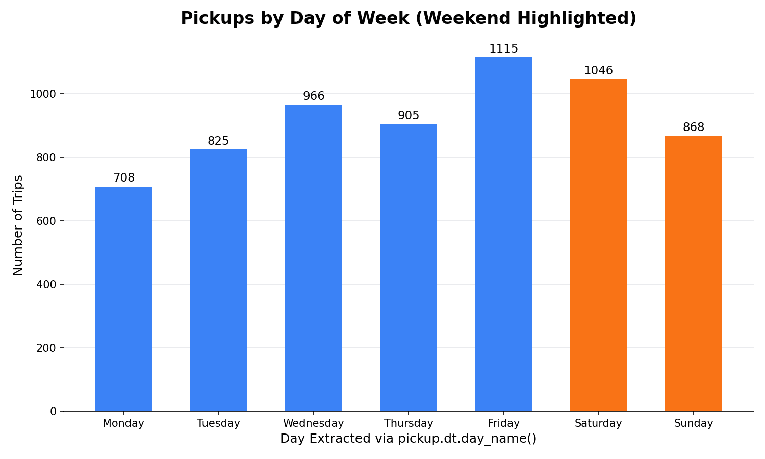
Friday is the single busiest day (1,115 trips), and Saturday isn't far behind (1,046). Monday is the quietest (708). The is_weekend flag alone captures a real chunk of that pattern: weekends (Saturday + Sunday combined) account for 1,914 trips versus 4,519 on weekdays.
Week Number, Quarter, and Semester
df['pickup_week'] = df['pickup'].dt.isocalendar().week
df['pickup_quarter'] = df['pickup'].dt.quarter

import numpy as np
df['pickup_semester'] = np.where(df['pickup_quarter'].isin([1, 2]), 1, 2)

df[['pickup', 'pickup_week', 'pickup_quarter', 'pickup_semester']].sample(5, random_state=42)
pickup pickup_week pickup_quarter pickup_semester
4092 2019-03-08 18:48:28 10 1 1
6282 2019-03-12 23:54:38 11 1 1
3237 2019-03-30 23:13:30 13 1 1
1891 2019-03-06 20:13:30 10 1 1
5010 2019-03-15 20:16:05 11 1 1.dt.isocalendar().week gives the ISO week number of the year (1-52/53). .dt.quarter gives which quarter of the year the date falls in (1-4). There's no built-in semester attribute, so it's built manually with np.where(): quarters 1 and 2 map to semester 1 (first half of the year), quarters 3 and 4 map to semester 2. np.where(condition, value_if_true, value_if_false) applies that logic to the whole column at once, the same pattern used for the categorical half of a Type 2 mixed variable in the previous post.
Because this dataset's dates all fall within late February and March, pickup_quarter and pickup_semester are 1 for every row here, again a property of this specific dataset's narrow date range, not the code. The mechanics are identical on a dataset that spans a full year.
Time Elapsed Since a Date
A common feature is "how long ago was this?", subtracting a date from today's date. pd.to_datetime('today') gives the current timestamp, and subtracting a datetime column from it produces a timedelta:
today = pd.to_datetime('today')
elapsed = today - df['pickup']

df['days_since_pickup'] = elapsed.dt.days
df[['pickup', 'days_since_pickup']].sample(5, random_state=42)
pickup days_since_pickup
4092 2019-03-08 18:48:28 2705
6282 2019-03-12 23:54:38 2701
3237 2019-03-30 23:13:30 2683
1891 2019-03-06 20:13:30 2707
5010 2019-03-15 20:16:05 2698elapsed is a timedelta64 column, a duration rather than a point in time. .dt.days pulls the whole-number day count out of it. These numbers are close to seven and a half years because this code actually ran on today's real date against real 2019 trip data.
To go from days to a rough month count, divide by 30:
df['months_since_pickup'] = elapsed.dt.days // 30
df[['pickup', 'days_since_pickup', 'months_since_pickup']].sample(5, random_state=42)
pickup days_since_pickup months_since_pickup
4092 2019-03-08 18:48:28 2705 90
6282 2019-03-12 23:54:38 2701 90
3237 2019-03-30 23:13:30 2683 89
1891 2019-03-06 20:13:30 2707 90
5010 2019-03-15 20:16:05 2698 89This is an approximation, not every month has exactly 30 days, but it's good enough for a feature that's meant to capture "roughly how many months ago", rather than a precise calendar calculation.
Extracting Time: Hour, Minute, Second
Everything so far pulled the date half apart. pickup also carries a time component, and it works the same way, through .dt:
df['pickup_hour'] = df['pickup'].dt.hour
df['pickup_minute'] = df['pickup'].dt.minute
df['pickup_second'] = df['pickup'].dt.second

df[['pickup', 'pickup_hour', 'pickup_minute', 'pickup_second']].sample(5, random_state=42)
pickup pickup_hour pickup_minute pickup_second
4092 2019-03-08 18:48:28 18 48 28
6282 2019-03-12 23:54:38 23 54 38
3237 2019-03-30 23:13:30 23 13 30
1891 2019-03-06 20:13:30 20 13 30
5010 2019-03-15 20:16:05 20 16 5If just the time portion is needed, without the date attached, .dt.time strips it out:
df['pickup_time_only'] = df['pickup'].dt.time
df[['pickup', 'pickup_time_only']].sample(5, random_state=42)
pickup pickup_time_only
4092 2019-03-08 18:48:28 18:48:28
6282 2019-03-12 23:54:38 23:54:38
3237 2019-03-30 23:13:30 23:13:30
1891 2019-03-06 20:13:30 20:13:30
5010 2019-03-15 20:16:05 20:16:05The hour alone is enough to see a real daily rhythm in the data:
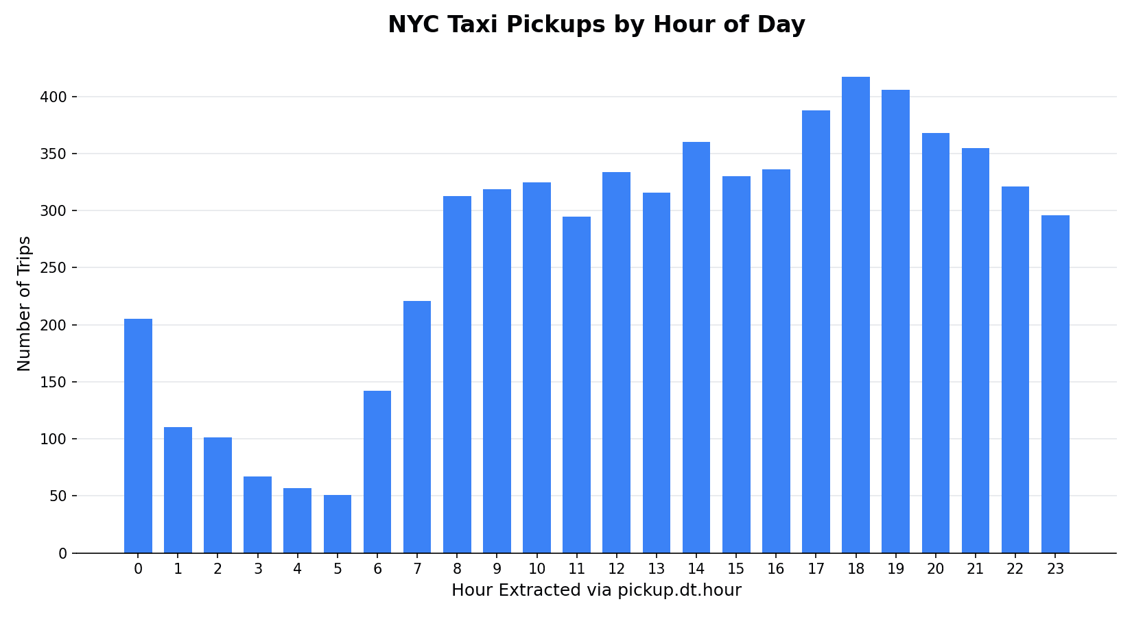
Pickups bottom out around 4-5 AM (50-57 trips) and climb steadily through the day, peaking at 6 PM with 417 trips, right in line with the evening rush hour a New Yorker would expect. This is exactly the kind of pattern a raw timestamp string can't expose, but .dt.hour makes trivial to compute and trivial for a model to use.
Time Elapsed Between Two Timestamps
The dataset also has dropoff, so subtracting one timestamp column from another gives a real, row-by-row duration, in this case, trip length:
df['trip_duration'] = df['dropoff'] - df['pickup']
df[['pickup', 'dropoff', 'trip_duration']].sample(5, random_state=42)
pickup dropoff trip_duration
4092 2019-03-08 18:48:28 2019-03-08 18:59:34 0 days 00:11:06
6282 2019-03-12 23:54:38 2019-03-13 00:03:34 0 days 00:08:56
3237 2019-03-30 23:13:30 2019-03-30 23:33:39 0 days 00:20:09
1891 2019-03-06 20:13:30 2019-03-06 20:27:10 0 days 00:13:40
5010 2019-03-15 20:16:05 2019-03-15 20:30:58 0 days 00:14:53trip_duration is a timedelta64 column again, same as elapsed earlier, just measured between two real timestamps instead of against today. .dt.days only gives whole days, which is too coarse for a trip that lasts minutes. For finer units, divide the timedelta by np.timedelta64(1, <unit>):
df['trip_seconds'] = df['trip_duration'] / np.timedelta64(1, 's')
df['trip_minutes'] = df['trip_duration'] / np.timedelta64(1, 'm')

df[['pickup', 'dropoff', 'trip_seconds', 'trip_minutes']].sample(5, random_state=42)
pickup dropoff trip_seconds trip_minutes
4092 2019-03-08 18:48:28 2019-03-08 18:59:34 666.0 11.100000
6282 2019-03-12 23:54:38 2019-03-13 00:03:34 536.0 8.933333
3237 2019-03-30 23:13:30 2019-03-30 23:33:39 1209.0 20.150000
1891 2019-03-06 20:13:30 2019-03-06 20:27:10 820.0 13.666667
5010 2019-03-15 20:16:05 2019-03-15 20:30:58 893.0 14.883333Dividing a timedelta by np.timedelta64(1, 'm') converts every value into "how many minutes is this", as a plain float. Swap 'm' for 's', 'h', or 'D' for seconds, hours, or days instead.
Across all 6,433 trips, trip_minutes averages 14.3 minutes, with the longest trip in the dataset running 107.7 minutes (from 2019-03-05 07:23:49 to 2019-03-05 09:11:29), and the shortest recorded at 0 minutes. A duration column like this, computed once, is often more useful to a model directly than the two raw timestamps it came from.
Summary Cheat Sheet
| Task | Code |
|---|---|
| Convert text to datetime | pd.to_datetime(df['col']) |
| Year / month / day | .dt.year / .dt.month / .dt.day |
| Month name | .dt.month_name() |
| Day of week (number / name) | .dt.dayofweek (0 = Monday) / .dt.day_name() |
| Is weekend | .dt.day_name().isin(['Saturday', 'Sunday']) |
| Week number / quarter | .dt.isocalendar().week / .dt.quarter |
| Semester | np.where(df['col'].dt.quarter.isin([1, 2]), 1, 2) |
| Hour / minute / second | .dt.hour / .dt.minute / .dt.second |
| Time only (no date) | .dt.time |
| Elapsed time between two dates | date2 - date1 gives a timedelta64; use .dt.days for whole days |
| Elapsed time in other units | timedelta_col / np.timedelta64(1, 's' | 'm' | 'h' | 'D') |
What's Next?
This post covered pulling structured features out of date and time columns: converting text to datetime64 with pd.to_datetime(), extracting date parts (year, month, day, day of week, weekend flag, week, quarter, semester), extracting time parts (hour, minute, second), and computing elapsed time between two timestamps with timedelta and np.timedelta64. Together with the previous post on mixed variables, that closes out the common "messy raw column" problems feature engineering has to deal with before a model ever sees the data.