Ch.33: Z-Score Method for Outlier Detection and Removal

Inspired by: YouTube

In the previous post, we introduced the foundational concepts of outliers: why they distort model performance, when to remove vs. keep them, and the taxonomy of handling techniques. In this post, we cover our first concrete technique: the Z-Score Method (also known as the 3-Sigma / Standard Deviation Rule) for detecting and removing outliers.

Core Assumption: Normality Requirement

Before applying the Z-Score method to any column, there is one non-negotiable prerequisite:

The feature column MUST follow a Normal (Gaussian) distribution, or at least be reasonably close to a bell curve.

If a column is heavily skewed (left-skewed or right-skewed), the mean $\mu$ and standard deviation $\sigma$ themselves become corrupted by tail values, invalidating the Z-Score boundary calculations. Skewed distributions should be handled using the IQR Proximity Rule, which will be covered in the next post.

The Mathematics of the Z-Score Rule

In a standard normal distribution $\mathcal{N}(\mu, \sigma^2)$, data points cluster symmetrically around the mean $\mu$ according to the 68-95-99.7 Empirical Rule:

• $\mu \pm 1\sigma$ contains 68.27% of all observations.
• $\mu \pm 2\sigma$ contains 95.45% of all observations.
• $\mu \pm 3\sigma$ contains 99.73% of all observations.

Lower Boundary = μ - 3 * σ
Upper Boundary = μ + 3 * σ

Any observation lying beyond $3\sigma$ from the mean accounts for fewer than 0.27% of samples under normal random variation. Statisticians treat values outside this range as statistical anomalies.

Converting Raw Feature Values to Z-Scores

The Z-score represents the number of standard deviations an individual observation $x_i$ lies away from the population mean $\mu$:

$Z_i = \frac{x_i - \mu}{\sigma}$

• A Z-score of 0 means the observation equals the mean.
• A Z-score of +2.5 means the observation lies 2.5 standard deviations above the mean.
• A Z-score of -3.2 means the observation lies 3.2 standard deviations below the mean.

Checking whether a feature value falls outside $[\mu - 3\sigma, \mu + 3\sigma]$ is mathematically identical to checking whether its absolute Z-score is greater than 3:

$\text{Outlier Condition: } |Z_i| > 3 \iff x_i < (\mu - 3\sigma) \quad \text{or} \quad x_i > (\mu + 3\sigma)$

The advantage of converting data to Z-scores is scale standardization: regardless of whether you are measuring height in centimeters, salary in thousands, or CGPA on a 10-point scale, the outlier threshold remains fixed at $|Z| > 3$.

Hands-On Python Walkthrough: placement.csv Dataset

Let's test the Z-score method on a real placement dataset containing 1,000 student records with two numerical features: cgpa and placement_exam_marks.

import numpy as np
import pandas as pd
import matplotlib.pyplot as plt
import seaborn as sns
 
df = pd.read_csv('placement.csv')
df.head()

   cgpa  placement_exam_marks  placed
0  6.89                  26.0       1
1  8.00                  14.0       1
2  5.12                  31.0       1
3  7.42                  33.0       1
4  6.84                  51.0       1

Step 1: Normality Check

We first plot histograms with KDE curves to verify which columns follow a Gaussian distribution:

plt.figure(figsize=(14, 5))
 
plt.subplot(1, 2, 1)
sns.histplot(df['cgpa'], kde=True)
plt.title('CGPA Distribution (Normally Distributed)')
 
plt.subplot(1, 2, 2)
sns.histplot(df['placement_exam_marks'], kde=True)
plt.title('Placement Exam Marks (Right-Skewed)')
 
plt.show()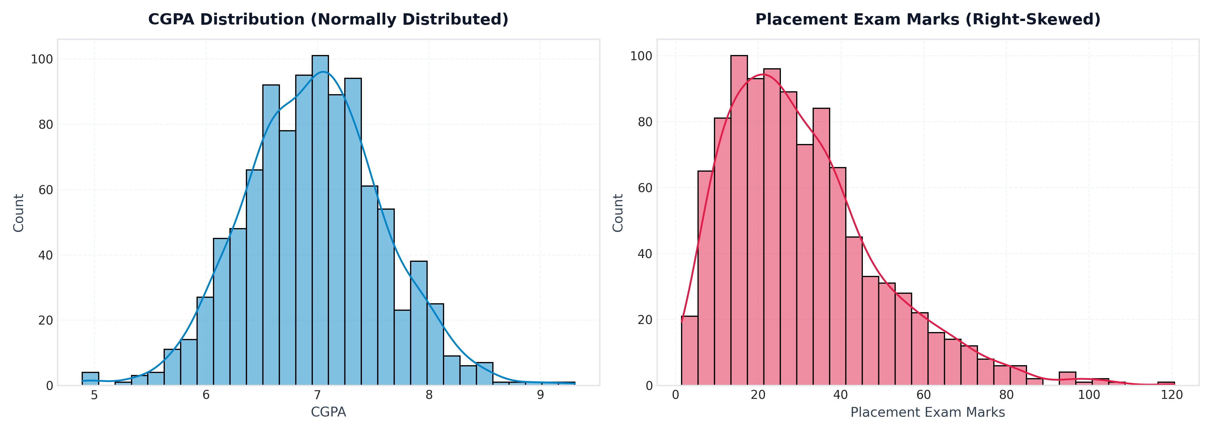

Key Observation

• cgpa: Displays a symmetric, classic bell-curve shape. Z-score method is valid here.
• placement_exam_marks: Heavily right-skewed (most students scored low, very few scored high). Z-score method CANNOT be used here (we will use IQR in the next post).

Step 2: Summary Statistics & Boundary Calculations

Next, we inspect the summary metrics of cgpa:

print("Mean CGPA:", df['cgpa'].mean())
print("Std CGPA :", df['cgpa'].std())
print("Min CGPA :", df['cgpa'].min())
print("Max CGPA :", df['cgpa'].max())

Mean CGPA: 6.96124
Std CGPA : 0.61589
Min CGPA : 4.89000
Max CGPA : 9.12000

Now we compute the upper and lower 3-sigma limits:

upper_limit = df['cgpa'].mean() + 3 * df['cgpa'].std()
lower_limit = df['cgpa'].mean() - 3 * df['cgpa'].std()
 
print("Upper Limit (μ + 3σ):", upper_limit)
print("Lower Limit (μ - 3σ):", lower_limit)

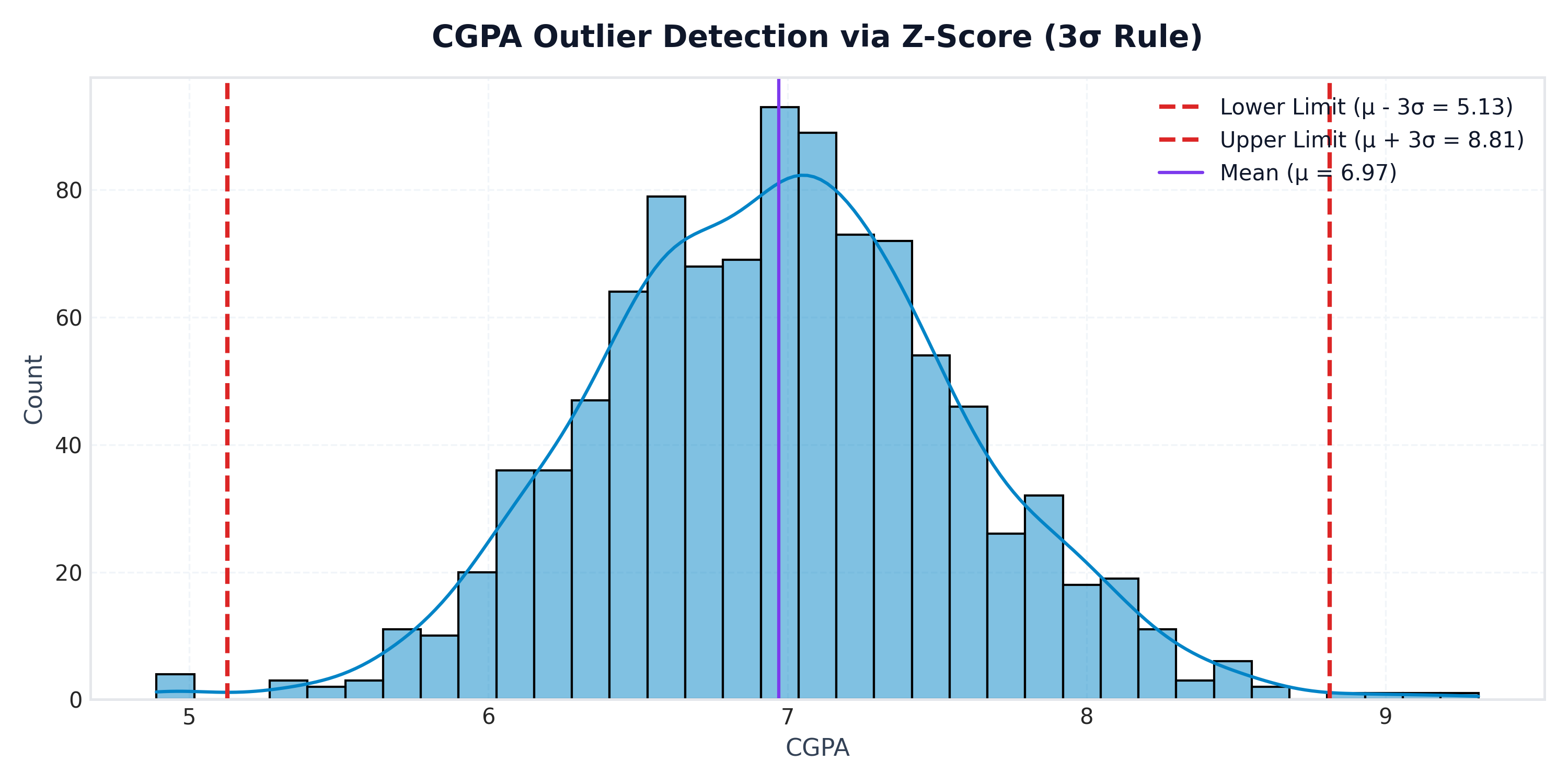
Upper Limit (μ + 3σ): 8.80893
Lower Limit (μ - 3σ): 5.11354

Any student with a CGPA greater than 8.80893 or lower than 5.11354 is classified as an outlier.

Step 3: Detecting Outlier Rows

We query the dataset to isolate observations outside these boundary limits:

# Filtering outliers using feature limits
outliers = df[(df['cgpa'] > upper_limit) | (df['cgpa'] < lower_limit)]
outliers

     cgpa  placement_exam_marks  placed
485  4.89                  16.0       0
496  4.90                  24.0       1
537  5.01                  52.0       0
995  8.95                  44.0       1
996  9.12                  65.0       1

Out of 1,000 students, exactly 5 observations violate the $3\sigma$ boundary: 3 on the lower tail ($4.89, 4.90, 5.01$) and 2 on the upper tail ($8.95, 9.12$).

Verification via Z-Score Standardization Formula

We can also calculate explicit Z-scores for every row to achieve the identical result:

# Create Z-score column
df['cgpa_zscore'] = (df['cgpa'] - df['cgpa'].mean()) / df['cgpa'].std()
 
# Filter where |Z| > 3
df[(df['cgpa_zscore'] > 3) | (df['cgpa_zscore'] < -3)]

     cgpa  placement_exam_marks  placed  cgpa_zscore
485  4.89                  16.0       0    -3.362985
496  4.90                  24.0       1    -3.346764
537  5.01                  52.0       0    -3.168161
995  8.95                  44.0       1     3.229081
996  9.12                  65.0       1     3.505105

Both conditions return the exact same 5 outlier rows.

Treatment Approach 1: Trimming (Dropping Outliers)

In Trimming, we drop rows containing outlier values and keep only observations within $[\mu - 3\sigma, \mu + 3\sigma]$:

# Trimming implementation
new_df_trimmed = df[(df['cgpa'] <= upper_limit) & (df['cgpa'] >= lower_limit)]
 
print("Original shape:", df.shape)
print("Trimmed shape :", new_df_trimmed.shape)

Original shape: (1000, 3)
Trimmed shape : (995, 3)

The dataset size shrinks from 1,000 rows to 995 rows, cleanly removing the 5 anomalous points.

Treatment Approach 2: Capping (Winsorization)

When dropping rows is undesirable because dataset size must be preserved, we apply Capping (also known as Winsorization).

Instead of deleting the 5 outlier rows, we clamp their values:

• Any CGPA $> 8.80893$ is replaced with $8.80893$.
• Any CGPA $< 5.11354$ is replaced with $5.11354$.

Implementation in Python via np.where

# Apply capping using nested np.where
df['cgpa_capped'] = np.where(
    df['cgpa'] > upper_limit,
    upper_limit,
    np.where(
        df['cgpa'] < lower_limit,
        lower_limit,
        df['cgpa']
    )
)
 
print("Original Min:", df['cgpa'].min(), "| Capped Min:", df['cgpa_capped'].min())
print("Original Max:", df['cgpa'].max(), "| Capped Max:", df['cgpa_capped'].max())
print("Final Dataset Shape:", df.shape)

Original Min: 4.89 | Capped Min: 5.11354
Original Max: 9.12 | Capped Max: 8.80893
Final Dataset Shape: (1000, 4)

Alternatively, np.clip performs the identical operation cleanly in one line:

# One-liner capping using np.clip
df['cgpa_capped'] = np.clip(df['cgpa'], a_min=lower_limit, a_max=upper_limit)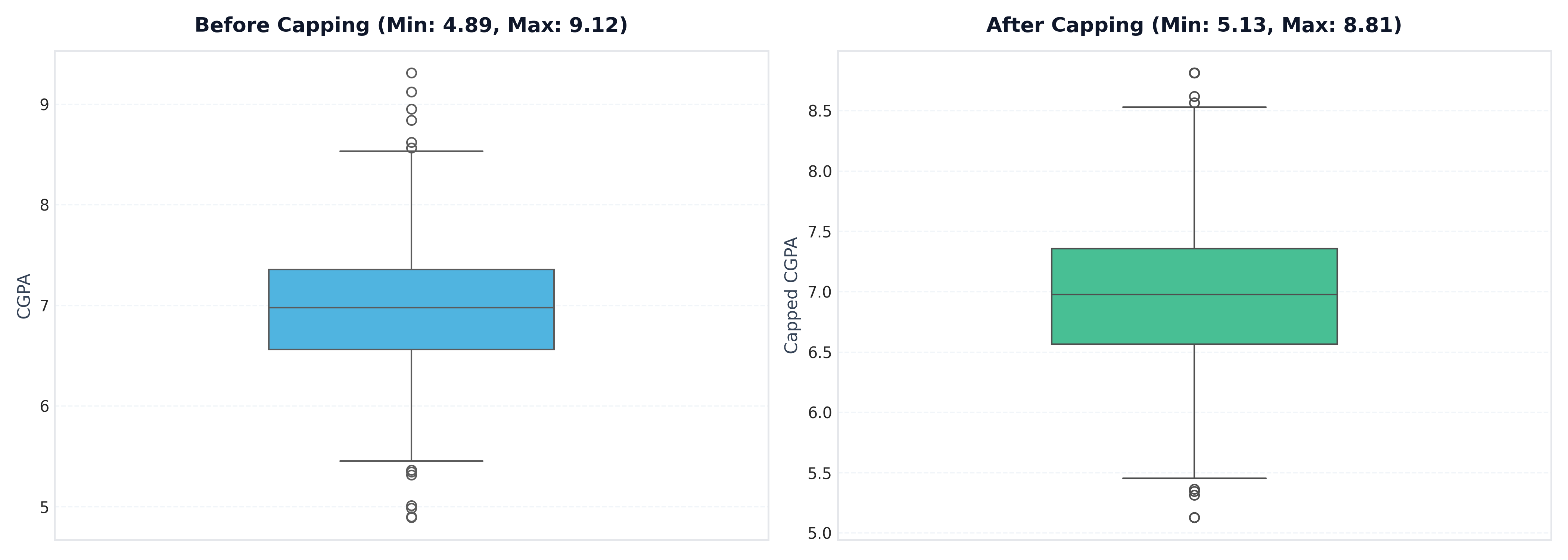

Why do points still appear outside the whiskers in the capped box plot? Seaborn and Matplotlib box plots compute whisker boundaries using the IQR rule ($Q_3 + 1.5 \times \text{IQR}$), NOT the Z-score $3\sigma$ rule. In a standard normal distribution, $1.5 \times \text{IQR}$ corresponds to roughly $\pm 2.7\sigma$. Because Z-score capping clamps extreme values at $\pm 3.0\sigma$, values clamped between $2.7\sigma$ and $3.0\sigma$ (e.g. 8.81 and 5.11) are correctly capped, but still sit slightly beyond the box plot's $2.7\sigma$ whisker boundary.

Summary & Key Takeaways

1. Prerequisite: The Z-score method strictly requires normally (or near-normally) distributed data. Do not apply it to skewed columns.
2. Boundary Threshold: Data points outside $\mu \pm 3\sigma$ (or $|Z| > 3$) are flagged as outliers under the 68-95-99.7 empirical rule.
3. Trimming vs. Capping:
   • Use Trimming (df[(df[col] >= lower) & (df[col] <= upper)]) if dataset size is large and dropping < 1% of rows does not impact training.
   • Use Capping (np.clip(df[col], lower, upper)) if sample size must be preserved or downstream models require consistent record counts.

In the next post, we will cover the IQR Proximity Rule to detect and treat outliers in skewed distributions where the Z-score method cannot be applied.