
Ch.30: KNN Imputer and Multivariate Imputation
Inspired by: YouTube
Every imputation technique so far, mean/median, arbitrary value, end of distribution, most frequent category, random sample, shares one trait: each column gets filled using only that column's own data. This post covers the first technique that breaks from that pattern, KNN Imputer, scikit-learn's implementation of multivariate imputation: filling a missing value by looking at the other columns in the row and borrowing from whichever training rows look most similar.
Univariate vs. Multivariate Imputation
Say a dataset has four columns and a row is missing a value in the first one. A univariate technique looks only at that first column's other, non-missing rows to decide what goes in the gap. A multivariate technique instead looks at columns two, three, and four on that same row, finds other rows whose columns two, three, and four look similar, and borrows their column-one values. KNN Imputer is the "similar rows" idea taken literally: treat each row as a point in space, and for a missing value, look at its k nearest neighbors and average what they have in that column.
Finding Neighbors When Some Values Are Missing
Ordinary Euclidean distance between two rows, each treated as a point with one coordinate per column, is the familiar formula:
That formula breaks the moment either row has a NaN in it, there's nothing to subtract. scikit-learn's KNNImputer uses a variant built for exactly this, nan_euclidean_distances, which does two things differently:
- Skip any coordinate where either row is missing. Only compute the squared difference over columns where both rows have a value.
- Rescale by how many columns actually got used, so that a distance computed from 2 present columns isn't unfairly small next to one computed from all 4. That rescaling factor is a weight, defined as:
which folds into the full distance as:
n_features is the total column count, n_present is how many of them weren't missing in either row for this particular pairwise comparison. This is exactly the "weight" scikit-learn's own docs name for this function, it inflates the sum-of-squares to compensate for using fewer terms, so distances stay roughly comparable whether a pair of rows shares 4 columns or only 2.
It's worth being precise about what this correction is actually for:
n_presentis a property of the pair being compared, not of one row being "more empty" in general, and the weight isn't there to penalize sparse-overlap pairs. A sum of fewer squared terms is, all else equal, a smaller number purely because fewer things are being added up, not because the rows are truly more similar. Left uncorrected, a pair sharing only one present column would tend to look artificially closer than a pair sharing all four, even if that one shared value disagrees a lot, and get wrongly picked as a "nearest" neighbor for the wrong reason. Scaling bywcorrects that bias by inflating the partial sum back up to roughly what a full-column comparison would have produced, so a thin-overlap pair no longer has an unfair advantage. It can still end up as the nearest neighbor, honestly, if the few values it does share are genuinely close.
A Worked Example on Real Titanic Rows
This uses the same Age / Pclass / Fare / Survived slice of Titanic the source notebook uses (more on that below). Row 766 in the training split is missing Age:
idx=766: Pclass=1.0, Fare=39.60, Age=NaNIts three nearest rows that do have an Age value, found by nan_euclidean_distances (equivalently, by hand with the formula above, n_features=3, and only Pclass/Fare present on every pair since Age is the very thing being compared to a NaN):
| idx | Pclass | Fare | Age | Distance to row 766 |
|---|---|---|---|---|
| 853 | 1.0 | 39.40 | 16.0 | 0.2449 |
| 583 | 1.0 | 40.13 | 36.0 | 0.6430 |
| 684 | 2.0 | 39.00 | 60.0 | 1.4283 |
Row 853 gets the shortest distance because it agrees with row 766 on Pclass exactly and is only 0.20 off on Fare, so , the is , since only Pclass and Fare were available to compare. Row 684 is farthest, it's a different Pclass entirely.
From Distance to a Filled Value
With n_neighbors=3, those three rows are the whole neighborhood. weights='uniform' would just average their Age values plainly, . weights='distance' instead weights each neighbor by , so closer rows count for more, and critically, the denominator is the sum of the weights, not a fixed count like 2 or 3:
Row 853, the closest match, pulls the estimate down toward 16 far more than the distant row 684 pulls it toward 60. Running KNNImputer(n_neighbors=3, weights='distance').fit_transform(X_train) on the real data confirms it: the actual imputed value for row 766 is 25.768, matching the hand calculation above exactly. It's worth being precise about that denominator: the source video's own manual walkthrough of a similar distance-weighted example divides by the neighbor count instead of the sum of the weights, which gives a different (wrong) number, the general formula for a weighted average is always , never .
Trying It on Titanic
Same setup as the source notebook: Age, Pclass, Fare as features, Survived as target, Age is the only column with missing values (about 19.9% of rows).
import numpy as np
import pandas as pd

from sklearn.model_selection import train_test_split
from sklearn.impute import KNNImputer, SimpleImputer
from sklearn.linear_model import LogisticRegression
from sklearn.metrics import accuracy_score

df = pd.read_csv('train.csv')[['Age', 'Pclass', 'Fare', 'Survived']]

X = df.drop(columns=['Survived'])
y = df['Survived']

X_train, X_test, y_train, y_test = train_test_split(X, y, test_size=0.2, random_state=2)
knn = KNNImputer(n_neighbors=3, weights='distance')
X_train_trf = knn.fit_transform(X_train)
X_test_trf = knn.transform(X_test)
lr = LogisticRegression()
lr.fit(X_train_trf, y_train)
y_pred = lr.predict(X_test_trf)
accuracy_score(y_test, y_pred)0.7094972067039106# Comparison with SimpleImputer --> mean
si = SimpleImputer()
X_train_trf2 = si.fit_transform(X_train)
X_test_trf2 = si.transform(X_test)
lr = LogisticRegression()
lr.fit(X_train_trf2, y_train)
y_pred2 = lr.predict(X_test_trf2)
accuracy_score(y_test, y_pred2)0.6927374301675978One call to fit_transform, KNNImputer fits its own internal nearest-neighbor structure on X_train and fills every missing Age using the worked-example logic above, in parallel for every row that needs it. .transform(X_test) reuses that same fitted structure, test-set rows get filled using distances computed against the training rows, never against other test rows, the same train/test separation discipline as every other imputation technique in this series. On this split, KNNImputer edges out SimpleImputer's mean by about 1.7 points, 70.95% versus 69.27%.
Tuning n_neighbors and weights
n_neighbors and weights are the two knobs, and there's no formula for the right n_neighbors, it's found by trying values and checking test accuracy, same as any other hyperparameter:
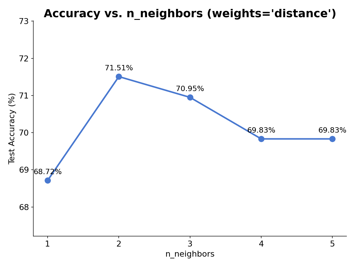
k=2 happens to edge out k=3 on this particular split, 71.51% versus 70.95%, and the curve is not monotonic in either direction, too few neighbors means each estimate leans on very little evidence, too many starts pulling in rows that aren't actually similar. weights matters too: switching the n_neighbors=3 run from 'distance' to 'uniform' drops accuracy slightly, 70.95% down to 70.39%, plain averaging lets a distant, less-relevant neighbor pull the estimate just as hard as a close one.
Does KNN Actually Preserve Relationships Between Columns?
Every univariate technique in this series has carried the same disadvantage: filling a column using only its own values ignores whatever relationship that column has with the others, and random sample imputation's .cov() check measured exactly that damage by keeping the original column and the imputed one side by side in the same DataFrame and calling .cov() once. Same move here: Age (still has its gaps) stays put, and Age_knn / Age_mean sit next to it as new columns, so one .corr() call shows every relationship, and every state, at once:
combined = X_train.copy()
combined['Age_knn'] = X_train_knn['Age']
combined['Age_mean'] = X_train_mean['Age']
combined = combined[['Pclass', 'Fare', 'Age', 'Age_knn', 'Age_mean']]

combined.corr()| Pclass | Fare | Age | Age_knn | Age_mean | |
|---|---|---|---|---|---|
| Pclass | 1.000 | -0.559 | -0.380 | -0.365 | -0.339 |
| Fare | -0.559 | 1.000 | 0.096 | 0.090 | 0.091 |
| Age | -0.380 | 0.096 | 1.000 | 1.000 | 1.000 |
| Age_knn | -0.365 | 0.090 | 1.000 | 1.000 | 0.937 |
| Age_mean | -0.339 | 0.091 | 1.000 | 0.937 | 1.000 |
The Pclass and Fare rows are the honest comparison, Age, Age_knn, and Age_mean are each correlated against a column that was never missing, so every cell in those two rows uses the full row count and is directly comparable to the others. Reading across: Age↔Pclass is -0.380 originally, mean imputation mutes it to -0.339, every missing Age becomes the exact same number regardless of Pclass, and KNN lands closer at -0.365, precisely because each fill used that row's own Pclass and Fare. But Age↔Fare tells a less clean story, 0.096 originally, KNN moves it to 0.090, mean to 0.091, KNN is not the closer of the two here even though Fare was one of the columns it used to pick each fill. Multivariate imputation doesn't guarantee every relationship improves, this split is a clear win for Age↔Pclass and a wash on Age↔Fare.
The Age / Age_knn / Age_mean block in the top-left of that 3×3 corner is the same gotcha Ch.29 ran into: every cell reads 1.000 because .corr() drops rows where either column is missing, and on every row where Age isn't missing, Age_knn and Age_mean are defined to equal it exactly, so those cells are quietly comparing Age's non-missing subset to a copy of itself. Age_knn↔Age_mean is the one cell in that corner not poisoned by that trick, neither column has any gaps left, so it uses every row, and it lands at 0.937, not 1.000. That number is the direct measure of how much the two imputation methods actually agree with each other: high, because most rows were never missing and both columns equal the real Age there, but not perfect, because on the ~20% of rows that were missing, KNN's per-row neighbor average and mean's single fixed constant rarely land on the same number twice.
Advantages and Disadvantages
- Advantage: generally more accurate fills than any univariate technique, because it uses more information, the values in the other columns of that same row, rather than only the target column's own distribution.
- Disadvantage: computationally expensive. Filling one missing value means computing a distance from that row to every other row in the training set, then sorting to find the nearest
k. That cost scales with the size of the dataset, not just the number of missing values. - Disadvantage: memory-heavy at deployment, and for a different reason than random sample imputation's version of the same problem.
KNNImputer.transform()on a brand-new incoming row needs to compute its distance against the entire training set stored inside the fitted object, so the whole training set has to live on the production server, not just a couple of summary numbers. That's slower and heavier than any technique covered so far in this series. - Good fit for: small to medium-sized datasets, where the extra computation at fit/transform time is cheap enough to be worth the accuracy gain, and the full training set isn't too large to keep in memory on the serving side.
Summary Cheat Sheet
| Aspect | KNN Imputer |
|---|---|
| scikit-learn | sklearn.impute.KNNImputer |
| Key params | n_neighbors (tune by trying values), weights ('uniform' or 'distance') |
| Distance metric | nan-aware Euclidean, rescaled by n_features / n_present per pair of rows |
| Use when | dataset is small/medium, better accuracy than univariate methods is worth the extra compute and memory |
| Avoid when | dataset is large (slow fit/transform), or the production server can't hold the full training set in memory |
What's Next?
KNNImputer fills a gap by borrowing from similar rows. The next post covers Iterative Imputer, a different multivariate approach that instead treats each column-with-missing-values as a regression target, predicted from the other columns, and repeats that process in rounds until the filled values stabilize.