Ch.56: AdaBoost From Scratch in Code

Inspired by: YouTube

The previous post derived AdaBoost's α formula and its weight-update mechanics on paper. This post is the code companion: the same source notebook, now built stage by stage in actual sklearn and pandas, so you can see exactly what each formula looks like as a line of code instead of a hand derivation. Along the way there's a genuinely useful bug in the notebook's third stage worth understanding, since it shows what actually goes wrong if you get the bookkeeping between stages wrong.

1. The Dataset

The notebook builds a small 10-row, two-feature toy dataset by hand rather than loading one, specifically so every intermediate number stays checkable:

df = pd.DataFrame()
df['X1'] = [1,2,3,4,5,6,6,7,9,9]
df['X2'] = [5,3,6,8,1,9,5,8,9,2]
df['label'] = [1,1,0,1,0,1,0,1,0,0]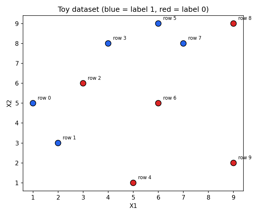

It's deliberately not linearly separable, no single straight line cleanly splits blue from red, which is the whole reason a single decision stump can't solve this in one shot and boosting needs multiple stages.

2. Stage 1: Train, Predict, Score

Every row starts at an equal weight, 1/n:

df['weights'] = 1 / df.shape[0]  # 0.1 for every row

Then a depth-1 stump (a decision stump, by definition) is trained on the raw data:

from sklearn.tree import DecisionTreeClassifier
dt1 = DecisionTreeClassifier(max_depth=1)
X = df.iloc[:, 0:2].values
y = df.iloc[:, 2].values
dt1.fit(X, y)
df['y_pred'] = dt1.predict(X)

This first stump splits on X2 <= 2.5, and gets 3 of the 10 rows wrong. Since all weights are still equal at 0.1, the error is the count of misclassified rows times 0.1: 0.1 + 0.1 + 0.1 = 0.3, plugged straight into the α formula from the last post:

def calculate_model_weight(error):
    return 0.5 * np.log((1 - error) / error)
 
alpha1 = calculate_model_weight(0.3)  # 0.4236489301936017

Worth noting: the notebook doesn't compute 0.3 from df['weights'] with a line of code, it's read off the printed y_pred column by eye (three rows visibly disagree with their label) and typed in directly as a literal. That's a fine shortcut for a teaching notebook where the whole dataset fits on one screen, but it also means the "error" step in this particular code isn't actually automated the way the formula in the last post implied it should be, it's manual pattern-matching against a printed table.

One practical aside from the video: on some datasets a stump can land at exactly 0 error, and 0.5 * log((1-0)/0) divides by zero. Worth knowing about if you're writing this by hand like the notebook does, but not something to actually work around yourself, scikit-learn's own AdaBoostClassifier already handles that edge case internally.

The decision boundary itself gets plotted with mlxtend.plotting.plot_decision_regions(X, y, clf=dt1), which is where the colored-region charts in this post come from, one call per stump, no manual meshgrid code needed.

3. Updating and Normalizing Weights

The weight-update function is a direct translation of the "multiply by e^alpha or e^-alpha" rule:

def update_row_weights(row, alpha=0.423):
    if row['label'] == row['y_pred']:
        return row['weights'] * np.exp(-alpha)
    else:
        return row['weights'] * np.exp(alpha)
 
df['updated_weights'] = df.apply(update_row_weights, axis=1)

Summed across all 10 rows, updated_weights comes to about 0.9165, not 1, so it gets normalized:

df['nomalized_weights'] = df['updated_weights'] / df['updated_weights'].sum()

(That's not a typo in this post, nomalized_weights missing the "r" is literally the column name in the source notebook. Harmless, but if you're following along and searching your own dataframe for normalized_weights you won't find it.)

Why Multiply by e^α, Not Just α?

The last post derived what α should equal but not why the update multiplies by e^alpha specifically instead of, say, adding α to the weight. The reasoning: e^x grows very slowly for small x and very steeply for large x. Since α is the model's trust score, a highly trustworthy stump (small error, large α) sits on the steep part of that curve, so its correction to the weights is aggressive, it punishes its own mistakes hard and rewards its correct calls hard. A weak stump (error close to 0.5, α close to 0) sits near the flat part, so e^alpha is close to 1 and it barely moves the weights at all, appropriately, since a coin-flip model shouldn't get to reshape the next stage's training data much. The exponential isn't an arbitrary choice of "some increasing function", its curvature is what ties the size of the weight update to how much the model has actually earned that trust.

4. Up-Sampling, in Code

The cumulative-range trick from the last post becomes two cumulative-sum columns and a nested loop:

df['cumsum_upper'] = np.cumsum(df['nomalized_weights'])
df['cumsum_lower'] = df['cumsum_upper'] - df['nomalized_weights']
 
def create_new_dataset(data):
    indices = []
    for i in range(data.shape[0]):
        a = np.random.random()
        for index, row in data.iterrows():
            if row['cumsum_upper'] > a and a > row['cumsum_lower']:
                indices.append(index)
    return indices
 
index_values = create_new_dataset(df)
second_df = df.iloc[index_values, [0, 1, 2, 3]]

np.random.random() here has no seed set anywhere in the notebook, so the exact resampled row indices are different every time this cell runs, on the original notebook and on any re-run of it. That's expected: up-sampling is supposed to be random. It does mean you shouldn't expect to reproduce the specific rows shown in any one run, only the shape of the outcome (heavily-weighted, i.e. previously-misclassified, rows show up more often).

5. Stage 2, and a Bug Worth Knowing About in Stage 3

Stage 2 repeats the exact same steps on second_df: train a fresh stump, get its error and α, update and normalize weights, up-sample into a third_df. Nothing new there.

Stage 3 is where the notebook's own code trips over itself. Right before training the third stump, it builds third_df from second_df's up-sampled weights, exactly as expected. But the actual training call reads:

dt3 = DecisionTreeClassifier(max_depth=1)
X = second_df.iloc[:, 0:2].values
y = second_df.iloc[:, 2].values
dt3.fit(X, y)

That's second_df again, the same X/y variables from stage 2, never reassigned to third_df. third_df gets built and then never used for training. Re-running this pipeline end to end makes the consequence obvious: since stage 3 trains on identical data to stage 2, it produces the same stump, with the same error and the same α, not a new, worse one:

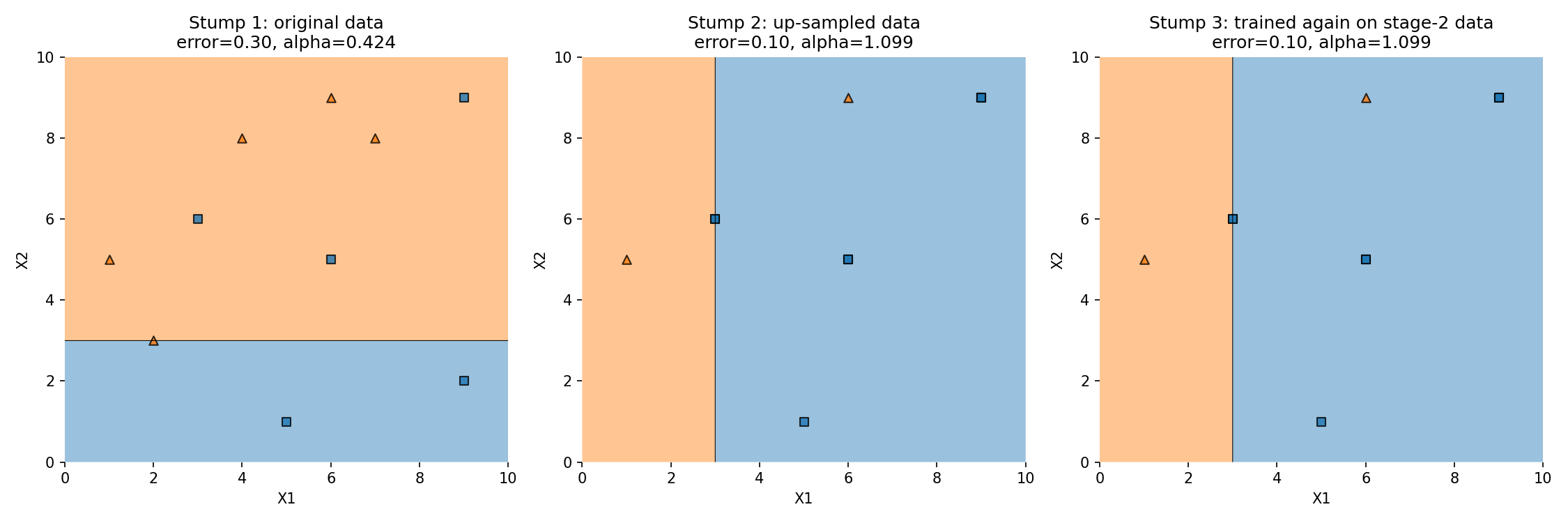
Panels 2 and 3 are pixel-identical, because they're the same decision boundary. That's the real cost of the bug: it's not that stage 3 becomes a bad model, it's that stage 3 becomes a redundant one, an ensemble member that adds no new information because it never saw the data it was supposed to correct for.

For contrast, the source notebook's own run reports an error of 0.7 for stage 3 (giving the negative α covered conceptually in the last post). Tracing the notebook further shows why that number is questionable rather than a real demonstration of an anti-correlated stump: the cell that counts stage 3's mistakes calls dt3.predict(X) with X still pointing at second_df's array, then compares that output against third_df's own labels, two dataframes with different rows in a different order. Counting "mismatches" between predictions for one dataset and labels from a different one isn't a real error rate, it's an artifact of the same variable-reuse bug compounding a second time. The 0.7 in the original video is best read as an illustrative number for explaining what a negative α means, not as this specific run's actual error.

6. Final Prediction

None of the above changes how the final ensemble vote is coded, once you have alpha1, alpha2, alpha3 and three trained stumps, prediction is just the sign of the weighted sum:

def predict(point):
    p1 = dt1.predict([point])[0]
    p2 = dt2.predict([point])[0]
    p3 = dt3.predict([point])[0]
    signed = lambda p: 1 if p == 1 else -1
    total = alpha1 * signed(p1) + alpha2 * signed(p2) + alpha3 * signed(p3)
    return np.sign(total)

For the query point (1, 5), all three stumps agree on class 1, so the sign of the sum is trivially positive: 0.4236 + 1.0986 + 1.0986 ≈ 2.62. For (9, 9), stump 1 predicts class 1 but stumps 2 and 3 (encoded as -1) both disagree, and since stumps 2 and 3 are, per the bug above, literally the same stump with the same α, their combined weight (1.0986 + 1.0986) easily outweighs stump 1's single vote: 0.4236 - 1.0986 - 1.0986 ≈ -1.77, sign negative. It reaches the same final answer as the last post's worked example, but for a different reason: not because a single stump with a large negative α flipped the vote, but because two identical, redundant stumps outvote the one that's actually different.

7. What to Take Away

• Every formula from the last post maps to a short, literal function: calculate_model_weight is the α formula, update_row_weights is the e^alpha/e^-alpha multiply, create_new_dataset is the cumulative-range draw.
• The notebook computes stage 1's error by reading a printed table and typing in a literal (0.3), not by summing a column in code, worth knowing if you expected the error step to be fully automated.
• Up-sampling uses an unseeded random draw, so re-running the notebook (or this post's code) will not reproduce the exact same resampled rows, only the same tendency to duplicate previously-misclassified rows.
• The notebook's stage 3 accidentally retrains on stage 2's data instead of the third_df it just built. The real consequence isn't a "bad" stump, it's a redundant one: training twice on the same data just gives back the same stump, contributing nothing new to the ensemble.
• The infamous "negative α" example from the last post's stage 3 traces back to a second variable-reuse bug when counting mistakes against the wrong dataframe, worth treating as an illustration of the concept rather than a literal number to trust.