Ch.55: AdaBoost, the α and Weight-Update Math

Inspired by: YouTube

The previous post covered AdaBoost's geometric picture: fit a decision stump, up-weight its mistakes, fit the next stump, repeat, then combine every stump's vote weighted by how good it was. That post left two things unexplained on purpose: how much say (α) each stump gets, and exactly how the up-sampling happens. Both come down to two formulas. This post derives them and then runs them on a real, small dataset so every number below is something you can recompute yourself.

1. Where We Left Off

Every row starts with an equal weight, $\frac{1}{n}$ for $n$ rows. Stage 1 trains a decision stump on the full, equally-weighted data. It gets some rows wrong, since a stump can only draw one axis-aligned split. Two things need to happen next: figure out how much this stump's opinion should count in the final vote (its α), and push its mistakes into the next stage's training data (up-sampling). This post is entirely about those two steps.

2. Error Isn't Just "How Many Rows Are Wrong"

Once a stump is fit, AdaBoost's error for that stage is the sum of the weights of the rows it misclassified, not a plain misclassification count. Early on, when every row has equal weight, this is basically the same as a normal error rate. But once weights start diverging in later stages, weight-sum error correctly gives heavily-weighted mistakes more influence than lightly-weighted ones, which is the whole point of carrying weights forward at all.

3. Deriving α: Why 0.5 * ln((1-error)/error)

α is how much a stump's vote counts in the final weighted sum. The video builds the formula from a simple thought experiment instead of just stating it: imagine three models.

• Model A is always right. Error rate 0.
• Model B is always wrong. Error rate 1 (100%).
• Model C is right exactly half the time. Error rate 0.5.

Which is most reliable? Model A, obviously, it should get the loudest vote. The more interesting question is between B and C. C looks better on paper (50% right beats 0% right), but B is actually more useful than it seems: a friend who is wrong every single time is just as informative as a friend who is right every single time, you just do the opposite of whatever they say. Flip B's answers and it becomes Model A. C, on the other hand, is a coin flip: agreeing with it or doing the opposite are equally useless, so C deserves zero weight in the vote, not positive and not negative.

That gives three anchor points for the α-vs-error curve:

• error near 0 → α should be a large positive number
• error = 0.5 → α should be 0
• error near 1 → α should be a large negative number (so its vote gets inverted, same logic as Model B)

is exactly the function that produces that shape. Plotting it against the three actual error rates that come up later in this post (0.3, 0.1, 0.7) makes the shape concrete:

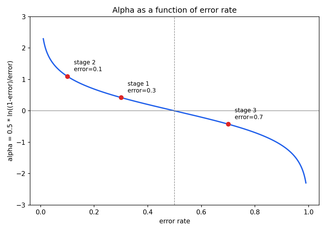
Note the third point: an error rate above 0.5 gives a negative α. That's not a bug, it's the Model B logic firing correctly: a stump that's wrong more often than not still carries information, just inverted.

4. A Real Stage 1, Worked End to End

To make every number checkable, this uses the exact toy dataset behind the source notebook: 10 rows, two features ($X_1$, $X_2$), a 0/1 label, every row starting at weight 0.1. A depth-1 stump fit on this data gets 3 of the 10 rows wrong. Since every row still has equal weight 0.1, the error is $3 \times 0.1 = 0.3$, giving:

5. Updating the Weights

Now push this stage's mistakes forward. Every row's weight gets multiplied by $e^{\alpha}$ if it was misclassified (boost it) or $e^{-\alpha}$ if it was correct (shrink it), and once every row has been updated this way the weights are renormalized by dividing each one by the new total, so they sum back to 1.

With $\alpha_1 = 0.4236$: a correctly classified row goes from 0.1 to $0.1 \times e^{-0.4236} \approx 0.0655$, a misclassified row goes from 0.1 to $0.1 \times e^{0.4236} \approx 0.1528$. Summed across all 10 rows those updated weights come to about 0.9165, not 1, which is exactly why the renormalization step matters:

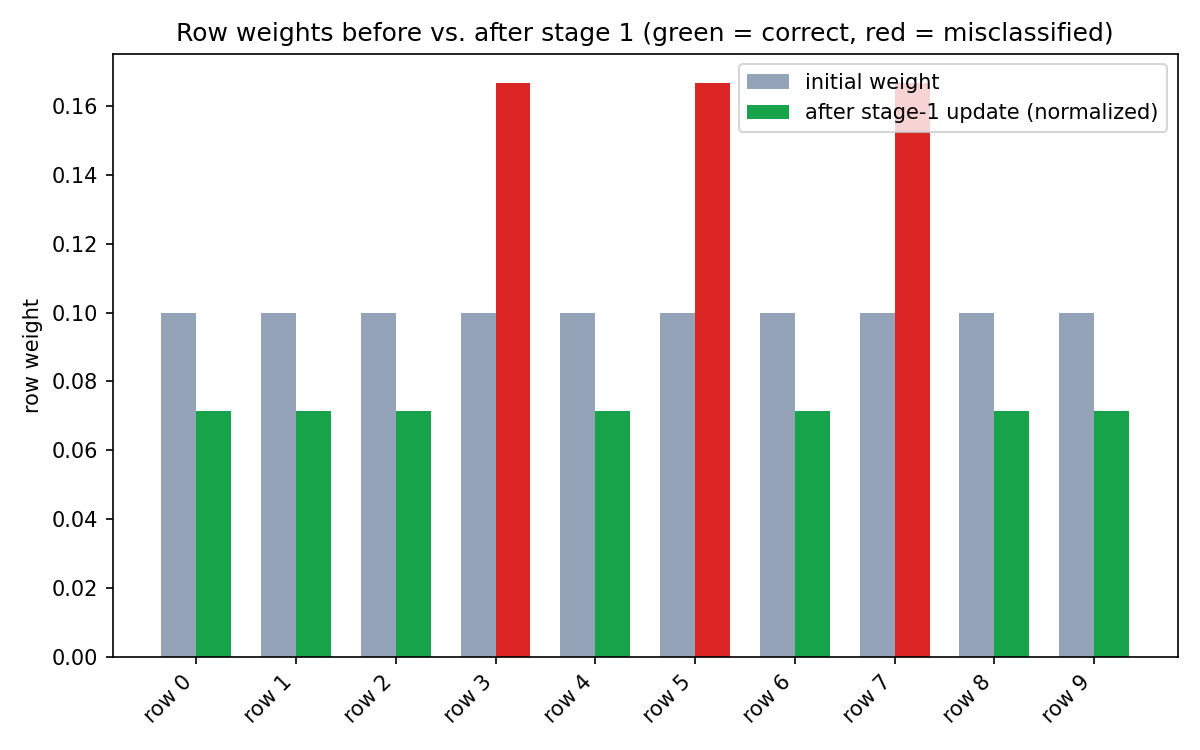
The 3 misclassified rows (red) went from 10% of the total weight each to about 16.7% each; the 7 correct ones (green) shrank to about 7.1% each. That's the entire "pay more attention to mistakes" mechanism: a plain multiply-and-renormalize, nothing fancier.

6. Up-Sampling: Turning Weights Into a New Dataset

A decision tree doesn't take a "weight" column as input, so AdaBoost can't just hand the next stump the reweighted table directly. Instead it builds a new physical dataset where heavily-weighted rows appear more than once, using weighted resampling:

1. Take the cumulative sum of the normalized weights, this gives every row a [lower, upper) slice of the 0-to-1 range, sized proportional to its weight.
2. Draw a uniform random number between 0 and 1.
3. Whichever row's slice the number lands in gets picked.
4. Repeat $n$ times to build a new dataset the same size as the original.

A row with a bigger slice (a misclassified row, after step 5) is proportionally more likely to get hit by a random draw, so it's more likely to show up multiple times, or at all, in the new dataset. Running this once (seeded, for reproducibility) on the stage-1 weights above:

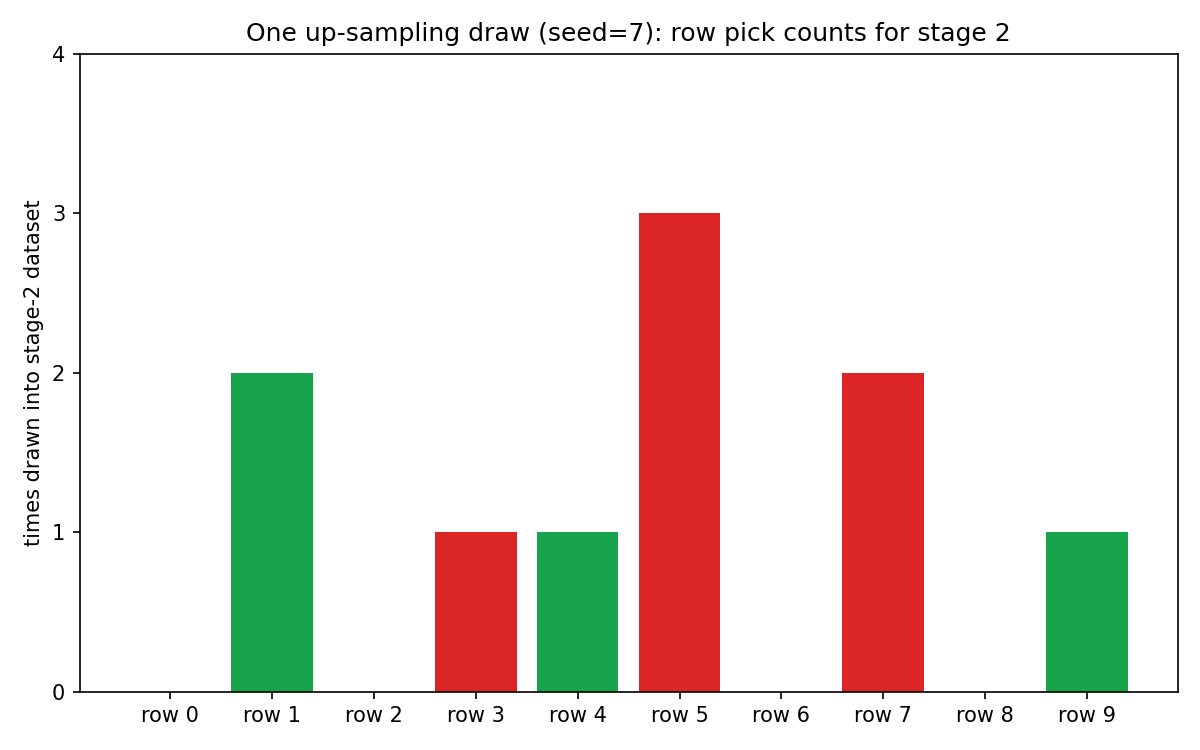
Worth being honest about what this chart actually shows: it's one random draw of 10 samples, not a guarantee. The 3 misclassified rows hold about 50% of the total weight after normalization ($3 \times 0.1667$), and in this particular draw they did end up with 6 of the 10 picks, close to that share, but a different random seed could easily land at 5 or 7. With only 10 rows the sampling noise is real; the expected frequency is what tracks the weight, not any single draw. Stage 2's stump then gets trained on this resampled dataset the same way stage 1's did, no weight column involved, since the reweighting has already been baked into which rows appear and how often.

7. Repeat, Then Combine

Stage 2 trains a fresh stump on the up-sampled data, gets its own error and its own α ($\alpha_2 \approx 1.0986$, from an error of 0.1 in the source notebook), and up-samples its own mistakes for stage 3. Stage 3's stump lands at an error of 0.7, above the 0.5 line from Section 3, so its α comes out negative: $\alpha_3 \approx -0.4236$. That's the Model B logic from the derivation showing up in a real run, not a hypothetical: a stump that's more often wrong than right is treated as anti-correlated with the truth, and its vote gets subtracted rather than added.

The notebook's own prediction check makes the payoff concrete. For a query point $(X1, X2) = (1, 5)$, all three stumps predict class 1:

For $(9, 9)$, stump 1 predicts class 1 but stumps 2 and 3 predict class 0 (read as -1 in the vote):

In the second case, stump 3's negative α combined with its "wrong-looking" -1 vote actually contributes positively toward the final +1... except here the final answer is -1, so it's stump 2's large $\alpha_2 = 1.0986$ that dominates. Either way, the sign of the weighted sum, not a majority vote, is what AdaBoost outputs, exactly the formula from the previous post.

8. What to Take Away

• Error at each stage is the sum of the weights of the misclassified rows, not a raw count, which is what makes later stages responsive to earlier reweighting.
• $\alpha = \frac{1}{2}\ln\left(\frac{1-\text{error}}{\text{error}}\right)$ falls out of a simple requirement: error near 0 → high positive α, error = 0.5 → zero α, error near 1 → large negative α (invert a consistently-wrong model rather than ignore it).
• Weight update is a plain multiply: $\times e^{\alpha}$ for misclassified rows, $\times e^{-\alpha}$ for correct ones, then renormalize so weights sum back to 1.
• Up-sampling turns weights into an actual resampled dataset via cumulative-range random draws, since a decision tree can't consume a weight column directly. It's probabilistic, not deterministic, so any single draw can look noisier than the underlying weights suggest, especially on small data.
• An error rate above 0.5 is not a broken stump, it produces a negative α, which flips that stump's vote in the final sum instead of discarding it.