
Ch.27: Numerical Imputation with Mean, Median, Arbitrary Value, and End of Distribution
Inspired by: YouTube
The last post covered Complete Case Analysis: dropping every row with a missing value, safe only when less than 5% of a column is missing and the data is MCAR. Most of the time neither condition holds, and the better move is imputation: filling the gaps in instead of throwing rows away. This post covers the first branch of that, univariate imputation for numerical columns, three separate techniques for deciding what value goes in the hole: mean/median, an arbitrary value, and a value pulled from the end of the distribution.
Univariate vs. Multivariate Imputation
Univariate imputation fills a column's missing values using only that column's own data, its mean, its median, or some other value derived from itself, with no reference to any other column. Multivariate imputation (KNN Imputer, Iterative Imputer, covered in later posts) uses the other columns to predict what the missing value should have been.
All three techniques below share the same shape: pick one number, and use it to fill in every missing value in the column. What differs is how that number gets picked, and each choice comes with its own tradeoff between simplicity and how badly it distorts the data.
The Dataset
This post uses the Titanic dataset, with age, fare, family (siblings/spouses plus parents/children aboard, sibsp + parch), and survived as the target.
import pandas as pd
import numpy as np
from sklearn.model_selection import train_test_split

df = pd.read_csv('https://raw.githubusercontent.com/mwaskom/seaborn-data/master/titanic.csv')
df['family'] = df['sibsp'] + df['parch']
df = df[['age', 'fare', 'family', 'survived']]

X = df.drop(columns='survived')
y = df['survived']
X_train, X_test, y_train, y_test = train_test_split(X, y, test_size=0.2, random_state=2)
X_train.shape, X_test.shape
((712, 3), (179, 3))age already has real missing values in this dataset, and fare doesn't, so 5% of fare gets randomly nulled out to demonstrate imputation on a column with light missingness too:
missing_idx = X_train.sample(frac=0.05, random_state=2).index
X_train.loc[missing_idx, 'fare'] = np.nan

X_train.isnull().mean() * 100
age 20.79
fare 5.06
family 0.00
dtype: float64As with CCA, statistics used for filling in values always come from the training set only. Whatever gets computed on X_train gets reused to transform X_test, never the other way around, otherwise information from the test set leaks into training.
Technique 1: Mean and Median Imputation
The simplest option: replace every missing value in a column with that column's own mean or median.
Which one to use comes down to the shape of the distribution. If a column is roughly normally distributed, mean, median, and mode all sit close together, so mean is the natural choice. If it's skewed, the mean gets pulled toward the tail while the median stays put, so median is the safer pick.
mean_age = X_train['age'].mean()
median_age = X_train['age'].median()
mean_fare = X_train['fare'].mean()
median_fare = X_train['fare'].median()

X_train['age'].skew(), X_train['fare'].skew()
(0.33, 4.59)age is close to normal (skew near 0), while fare is heavily right-skewed, a small number of passengers paid far more than everyone else. That shows up directly in the two sets of statistics:
mean_age = 29.79     median_age = 28.75
mean_fare = 32.18     median_fare = 14.25
For age, mean and median are less than a year apart. For fare, they're worlds apart: the mean gets dragged up to 32.18 by the small cluster of expensive first-class tickets, while the median of 14.25 reflects what a typical passenger actually paid. Filling fare's missing values with the mean here would insert a value most passengers never paid anywhere close to.
Advantages
- Trivial to implement, one
.fillna()call. - Works well when missingness is low, under roughly 5%, same threshold as CCA.
Disadvantages
- Distorts the distribution's shape. Piling extra mass onto a single value changes the PDF.
- Shrinks the variance, since every filled-in value sits exactly at the center, with zero spread of its own.
- Distorts correlation with other columns, since the filled-in rows contribute a constant instead of a value that actually correlates with the other columns.
- Manufactures outliers that weren't there before. Piling values onto the median squeezes the IQR, so the whiskers of a boxplot pull inward, and real, ordinary values near the old edges now fall outside them.
Seeing the Distortion
X_train['age_median'] = X_train['age'].fillna(median_age)
X_train['age_mean'] = X_train['age'].fillna(mean_age)
X_train['fare_median'] = X_train['fare'].fillna(median_fare)
X_train['fare_mean'] = X_train['fare'].fillna(mean_fare)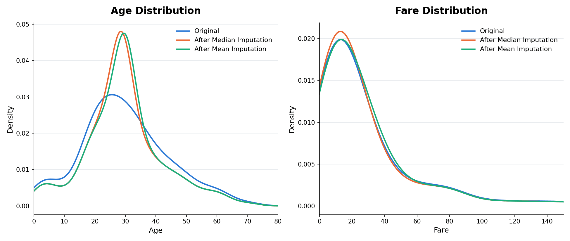
Both imputed curves grow a sharper peak right at the fill value, exactly where the extra density piles up. The effect on variance is measurable:
X_train['age'].var(), X_train['age_median'].var(), X_train['age_mean'].var()(204.35, 161.99, 161.81)Variance drops by about 20% just from filling in roughly a fifth of the column with a single constant. The correlation with family shifts too:
X_train['age'].corr(X_train['family'])       # -0.299
X_train['age_median'].corr(X_train['family']) # -0.243
Original: -0.299
After Median: -0.243That's the tradeoff CCA doesn't have: dropping rows preserves the shape of what's left, but imputation changes the shape of the column itself. It's an acceptable price only when missingness is low enough that the damage stays small, which is why the same 5% rule from CCA applies here too.
It Also Manufactures Outliers
A subtler side effect shows up in a boxplot. The IQR-based outlier rule flags anything outside Q1 - 1.5*IQR to Q3 + 1.5*IQR, and piling ~21% of age onto a single median value pulls Q1 and Q3 closer together, shrinking the IQR itself:
def iqr_bounds(s):
    Q1, Q3 = s.quantile(0.25), s.quantile(0.75)
    IQR = Q3 - Q1
    return Q1, Q3, IQR, Q1 - 1.5 * IQR, Q3 + 1.5 * IQR

iqr_bounds(X_train['age'].dropna())
iqr_bounds(X_train['age_median'])
Original: Q1=21.00 Q3=38.25 IQR=17.25 bounds=(-4.88, 64.12)
After Median: Q1=23.00 Q3=35.00 IQR=12.00 bounds=(5.00, 53.00)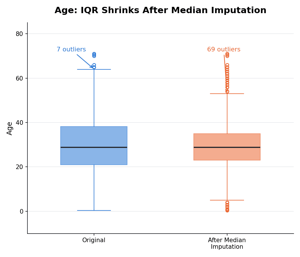
The upper bound drops from 64.12 to 53.00, and the lower bound rises from below zero to 5.00. Passengers in their late 50s and early 60s, who were never outliers to begin with, now fall outside the whiskers, and so does anyone genuinely aged under 5. The number of points an IQR rule would flag as outliers jumps from 7 to 69, none of which are actually anomalies, they're just ordinary values that got squeezed out by a shrinking box. Any downstream step that trims or caps outliers based on this boxplot would now be acting on manufactured noise instead of real ones.
The scikit-learn Way
Doing this by hand works for a one-off notebook, but a pipeline needs it as a proper transformer. Since age and fare need different strategies (median vs. mean), a ColumnTransformer routes each column to its own SimpleImputer:
from sklearn.impute import SimpleImputer
from sklearn.compose import ColumnTransformer

trf = ColumnTransformer([
    ('age_imputer', SimpleImputer(strategy='median'), ['age']),
    ('fare_imputer', SimpleImputer(strategy='mean'), ['fare']),
], remainder='passthrough')

trf.fit(X_train)
trf.named_transformers_['age_imputer'].statistics_
trf.named_transformers_['fare_imputer'].statistics_
age_imputer statistics_: [28.75]
fare_imputer statistics_: [32.18129231]Same numbers as the manual calculation, confirming the transformer learned the right values from X_train. Fitting happens once, on the training data; both X_train and X_test then get transformed with those same learned values:
X_train_trf = trf.transform(X_train)
X_test_trf = trf.transform(X_test)
The advantage of doing it this way over plain pandas is that the whole thing drops straight into a Pipeline, works with GridSearchCV, and ships to production without extra glue code.
Technique 2: Arbitrary Value Imputation
Instead of picking a value from inside the distribution, arbitrary value imputation fills every missing value with a fixed number that clearly doesn't belong in the data, something like 99, -1, or 9999. It's used far more often for categorical columns (filling with a placeholder like "Missing"), but it applies to numerical ones too.
The idea isn't to guess a plausible value, it's to mark which rows were missing in the first place, so the model can learn "this row had no data here" as its own signal.
Advantages
- Easy to apply, no statistics to compute.
- Flags missingness explicitly, giving the model a way to distinguish "was missing" from "had a real value."
Disadvantages
- Distorts the distribution, variance, and correlation far more aggressively than mean/median imputation, since the fill value sits outside the data's natural range instead of near its center.
X_train['age_99'] = X_train['age'].fillna(99)
X_train['age_minus1'] = X_train['age'].fillna(-1)

X_train['age'].var(), X_train['age_99'].var(), X_train['age_minus1'].var()
(204.35, 951.73, 318.09)Filling with 99 more than quadruples the variance, filling with -1 pushes it up by 55%, both far worse than the ~20% drop mean/median imputation caused. With scikit-learn, this is SimpleImputer with strategy='constant':
trf = ColumnTransformer([
    ('age_imputer', SimpleImputer(strategy='constant', fill_value=99), ['age']),
    ('fare_imputer', SimpleImputer(strategy='constant', fill_value=999), ['fare']),
], remainder='passthrough')
trf.fit(X_train)
Because of how much it distorts the data, this technique is used less often on numerical columns, and mostly matters when the goal really is to preserve a "was this missing" flag for the model rather than to fill in a realistic number.
Technique 3: End of Distribution Imputation
This is a more disciplined version of arbitrary value imputation. Instead of hand-picking a number like 99, the fill value is calculated to sit just past the tail of the column's own distribution:
- If the column is roughly normally distributed, use
mean + 3 * std. - If the column is skewed, use the IQR proximity rule:
Q3 + 1.5 * IQR.
eod_age = X_train['age'].mean() + 3 * X_train['age'].std()

Q1 = X_train['fare'].quantile(0.25)
Q3 = X_train['fare'].quantile(0.75)
IQR = Q3 - Q1
eod_fare = Q3 + 1.5 * IQR

eod_age, eod_fare
(72.67, 64.90)age (skew ≈ 0.33) gets the normal-distribution formula, landing at 72.67, well past the oldest typical passengers. fare (skew ≈ 4.59) gets the IQR rule instead, landing at 64.90.
X_train['age_eod'] = X_train['age'].fillna(eod_age)
X_train['age'].var(), X_train['age_eod'].var()
(204.35, 465.07)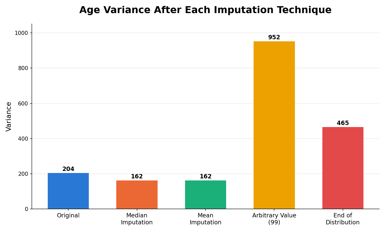
Lined up side by side, the pattern is clear: mean/median imputation shrinks variance slightly, while arbitrary value and end of distribution imputation both inflate it well past the original, arbitrary value the most since 99 sits even further from the data than the calculated tail value does.
Advantages and Disadvantages
Functionally the same as arbitrary value imputation, easy to apply, and it creates the same "this was missing" signal for the model. The disadvantages carry over too: distribution, variance, and correlation with other columns all shift, in this case even more than plain arbitrary value imputation for age. The upside over hand-picking 99 is that the fill value is derived from the data itself instead of guessed, so it's less likely to accidentally land inside the range of real values.
When to Use Which
Mean/median imputation and end of distribution/arbitrary value imputation aim at opposite goals, and the choice comes down to why the data is missing:
- If the data is Missing Completely At Random (MCAR) and the missing fraction is small, mean or median imputation is the safer choice, it does the least damage to the distribution.
- If there's reason to believe the data is not missing at random, arbitrary value or end of distribution imputation is more appropriate, since the goal shifts from "guess a realistic value" to "make sure the model can tell this row was incomplete."
Summary Cheat Sheet
| Technique | Fill Value | Use When |
|---|---|---|
| Mean Imputation | df[col].mean() | MCAR, <5% missing, roughly normal distribution |
| Median Imputation | df[col].median() | MCAR, <5% missing, skewed distribution |
| Arbitrary Value | a fixed out-of-range number, e.g. -1, 99 | data not MCAR, want an explicit "was missing" flag |
| End of Distribution | mean + 3*std or Q3 + 1.5*IQR | data not MCAR, want a calculated (not guessed) flag value |
What's Next?
This post covered the first two categories of univariate imputation for numerical data: mean/median imputation, which stays close to the original distribution but only works when little data is missing, and arbitrary value/end of distribution imputation, which sacrifices distribution shape in exchange for flagging which rows had missing data. The next posts in this series cover Random Sample Imputation, filling gaps with values randomly drawn from the column itself, and how to automatically select the best imputation technique for a given column instead of guessing.