
Ch.28: Categorical Imputation with Most Frequent Category and Missing Category
Inspired by: YouTube
The last post covered univariate imputation for numerical columns: mean/median, arbitrary value, and end of distribution. Categorical columns can't use any of those, there's no mean of "Mumbai", "Delhi", and "Kolkata". This post covers the categorical equivalent: filling missing values with the most frequent category, and, when that doesn't work, carving out a new "Missing" category instead.
Most Frequent Category (Mode) Imputation
The direct analogue of mean/median imputation for categorical data is mode imputation: replace every missing value with whichever category shows up most often in the column. A city column with Mumbai, Delhi, and Kolkata, where Mumbai is the most common, gets every missing row filled with Mumbai.
Mode exists for numerical columns too, technically nothing stops it from being computed there, but mean and median simply perform better on numerical data, so mode imputation is really a categorical-data technique in practice.
When It's Safe to Use
Two conditions, mirroring the ones from numerical imputation:
- The data is Missing Completely At Random (MCAR), same requirement as every other univariate technique in this series.
- One category clearly dominates the others. If
Mumbaishows up far more often thanDelhiorKolkata, filling gaps withMumbaibarely changes the column's shape. If the top categories are close in frequency, mode imputation forces an artificial winner and skews the column hard.
Advantages and Disadvantages
- Advantage: trivial to implement, a single
.fillna()call, fast enough to run in production without a second thought. - Disadvantage: it distorts the column's category proportions, and how badly depends entirely on whether condition 2 above holds. The example below shows both ends of that spectrum on the same dataset.
Trying It on a Real Dataset
This post uses the Ames housing dataset (Kaggle's "House Prices: Advanced Regression Techniques"), narrowed to three columns: GarageQual (garage quality) and FireplaceQu (fireplace quality), and SalePrice as the target. Both quality columns use the same five-point scale, worst to best: Po (Poor), Fa (Fair), TA (Typical/Average), Gd (Good), Ex (Excellent). A row's value is null when the house has no garage or no fireplace at all, there's nothing to rate. These two columns were picked deliberately, one has light missingness with a dominant category, the other has heavy missingness with no dominant category, which makes them a natural side-by-side test of when mode imputation works.
import pandas as pd
from sklearn.datasets import fetch_openml
from sklearn.model_selection import train_test_split

df = fetch_openml(name='house_prices', as_frame=True, parser='auto').frame
df = df[['GarageQual', 'FireplaceQu', 'SalePrice']]

X = df.drop(columns='SalePrice')
y = df['SalePrice']
X_train, X_test, y_train, y_test = train_test_split(X, y, test_size=0.2, random_state=2)

X_train.isnull().mean() * 100
GarageQual 5.57
FireplaceQu 47.69
dtype: float64GarageQual sits comfortably in the "safe" range. FireplaceQu is missing on nearly half the rows, immediately a red flag for mode imputation regardless of how the categories are distributed.
Checking Whether Missingness Relates to the Target
Before picking a technique, it's worth checking whether missingness itself carries information, comparing SalePrice for rows where the column is present against rows where it's missing. SalePrice was dropped out of X_train for the split, so this check joins it back onto a separate frame rather than mutating X_train itself:
train_with_target = X_train.join(y_train)

for col in ['GarageQual', 'FireplaceQu']:
    present = train_with_target.loc[train_with_target[col].notna(), 'SalePrice']
    missing = train_with_target.loc[train_with_target[col].isna(), 'SalePrice']
    print(col, 'present:', present.median(), present.mean(), len(present))
    print(col, 'missing:', missing.median(), missing.mean(), len(missing))
The .loc line is doing two things at once: .loc[row_selector, column_selector] takes a row selector and a column selector, separated by a comma. train_with_target[col].notna() is the row selector, a boolean Series the same length as the table, True wherever that column isn't null and False wherever it is. 'SalePrice' is the column selector, just the one column to keep. Pandas keeps only the rows where the mask is True, then returns just SalePrice for those rows as a Series. present ends up as "the SalePrice values, but only from rows where col isn't missing." The missing line is the mirror image, .isna() is the exact opposite mask of .notna(), so it's "the SalePrice values, but only from rows where col is missing." Two groups, split by whether one column was recorded, both restricted to a different column's values, that's the comparison the KDE chart below is built on.
GarageQual present: median=167000, mean=184425 (n=1103)
GarageQual missing: median=100000, mean=104560 (n=65)

FireplaceQu present: median=190000, mean=215351 (n=611)
FireplaceQu missing: median=135000, mean=141182 (n=557)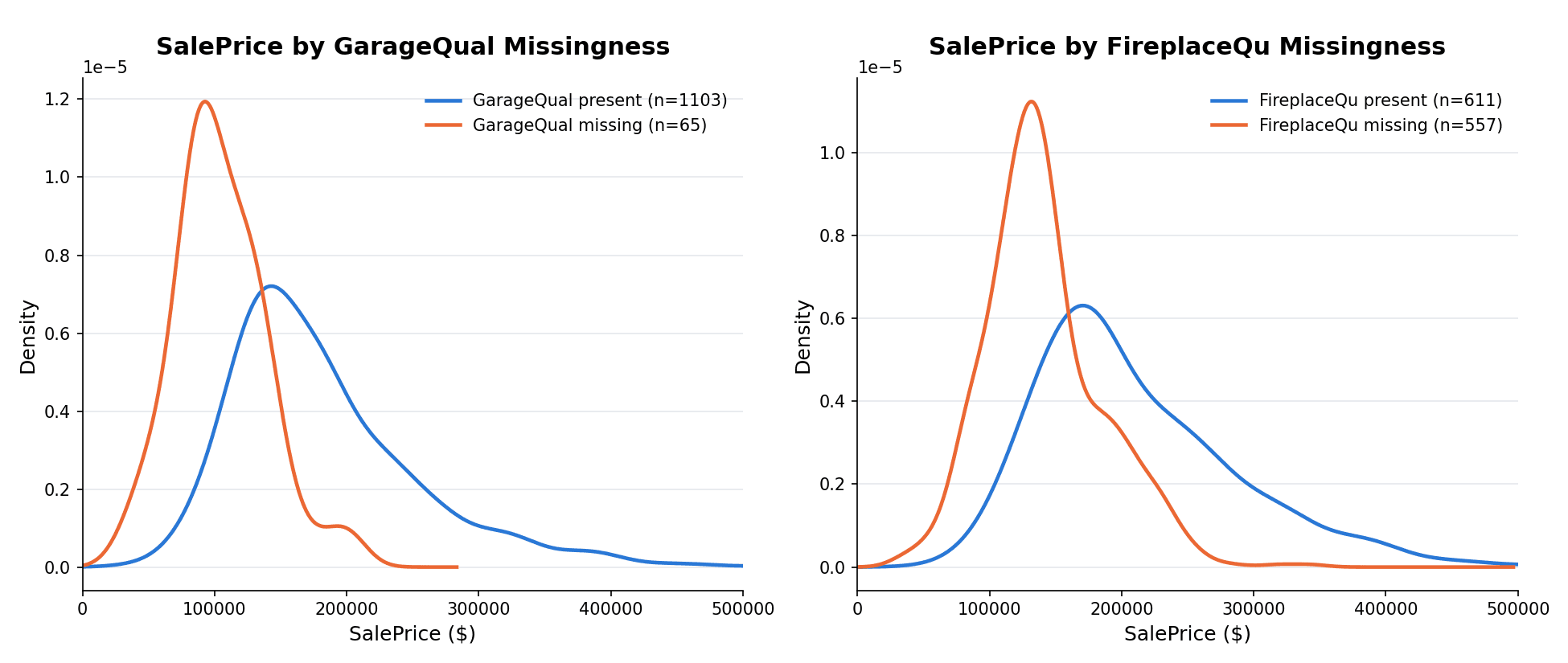
Both panels tell the same story: houses missing a value sell for meaningfully less, roughly 55,000 less for FireplaceQu. That's not a coincidence, in this dataset a null in GarageQual or FireplaceQu almost always means the house simply has no garage or no fireplace, and houses without those features tend to be smaller and cheaper. The missingness isn't random noise, it's meaningful information about the house itself, which is exactly the situation where a "Missing" category earns its keep: it isn't standing in for a guess, it's encoding a real fact.
Checking for a Dominant Category
X_train['GarageQual'].value_counts(normalize=True) * 100TA 95.10
Fa 3.72
Gd 1.00
Po 0.09
Ex 0.09X_train['FireplaceQu'].value_counts(normalize=True) * 100Gd 49.43
TA 41.24
Fa 4.09
Po 2.78
Ex 2.45GarageQual passes both conditions: TA dominates at 95%, nothing close to a tie. FireplaceQu fails condition 2 outright, Gd and TA are separated by only 8 points, nowhere near dominant.
Imputing and Comparing
mode_garage = X_train['GarageQual'].mode()[0]      # 'TA'
mode_fireplace = X_train['FireplaceQu'].mode()[0]  # 'Gd'

X_train['GarageQual_imputed'] = X_train['GarageQual'].fillna(mode_garage)
X_train['FireplaceQu_imputed'] = X_train['FireplaceQu'].fillna(mode_fireplace)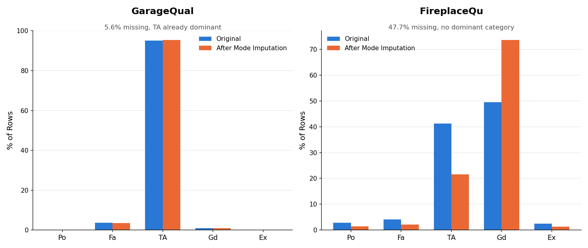
GarageQual's bars barely move, TA goes from 95.10% to 95.38%, imputation added a sliver on top of a category that already dominated. FireplaceQu tells the opposite story: Gd jumps from 49.43% to 73.54%, absorbing almost all of the missing 47.69% on top of its own share, while TA gets nearly cut in half, from 41.24% down to 21.58%. Neither number reflects reality, it's an artifact of forcing every unknown value into whichever category happened to be marginally ahead.
The scikit-learn Way
from sklearn.impute import SimpleImputer
from sklearn.compose import ColumnTransformer

trf = ColumnTransformer([
    ('garage_imputer', SimpleImputer(strategy='most_frequent'), ['GarageQual']),
    ('fireplace_imputer', SimpleImputer(strategy='most_frequent'), ['FireplaceQu']),
], remainder='passthrough')

trf.fit(X_train[['GarageQual', 'FireplaceQu']])
trf.named_transformers_['garage_imputer'].statistics_
trf.named_transformers_['fireplace_imputer'].statistics_
garage_imputer statistics_: ['TA']
fireplace_imputer statistics_: ['Gd']Same modes as the manual calculation. As with numerical imputation, strategy='most_frequent' is the scikit-learn equivalent, and fitting stays confined to X_train, with X_test transformed using those same learned categories.
Given the distortion on FireplaceQu, the answer to "should mode imputation be used here" is no, not because the code is wrong, but because the column fails both the MCAR-adjacent assumption of light missingness and the dominant-category requirement.
Missing Category Imputation
The fix for a column like FireplaceQu isn't a better guess, it's not guessing at all. Missing category imputation creates an entirely new category, typically named "Missing", and every null gets filled with that label instead of an existing one.
This is the direct categorical counterpart to arbitrary value imputation from the last post (99, -1, or a value at the tail of the distribution): instead of picking a plausible value, the goal is to flag which rows had no data, and let the model treat that as its own signal.
When to Use It
- Data is not MCAR, or there's no way to confirm that it is.
- Missingness is heavy and no category dominates, exactly
FireplaceQu's situation.
Advantages and Disadvantages
- Advantage: just as easy to implement as mode imputation, one
.fillna('Missing')call. - Disadvantage: minimal on its own, the main cost is that it isn't really informed imputation, it's an honest admission that the value is unknown, so a downstream model has to learn what to do with that category rather than being handed a plausible guess.
X_train['FireplaceQu_missing'] = X_train['FireplaceQu'].fillna('Missing')
X_train['FireplaceQu_missing'].value_counts(normalize=True) * 100
Missing 47.69
Gd 25.86
TA 21.58
Fa 2.14
Po 1.46
Ex 1.28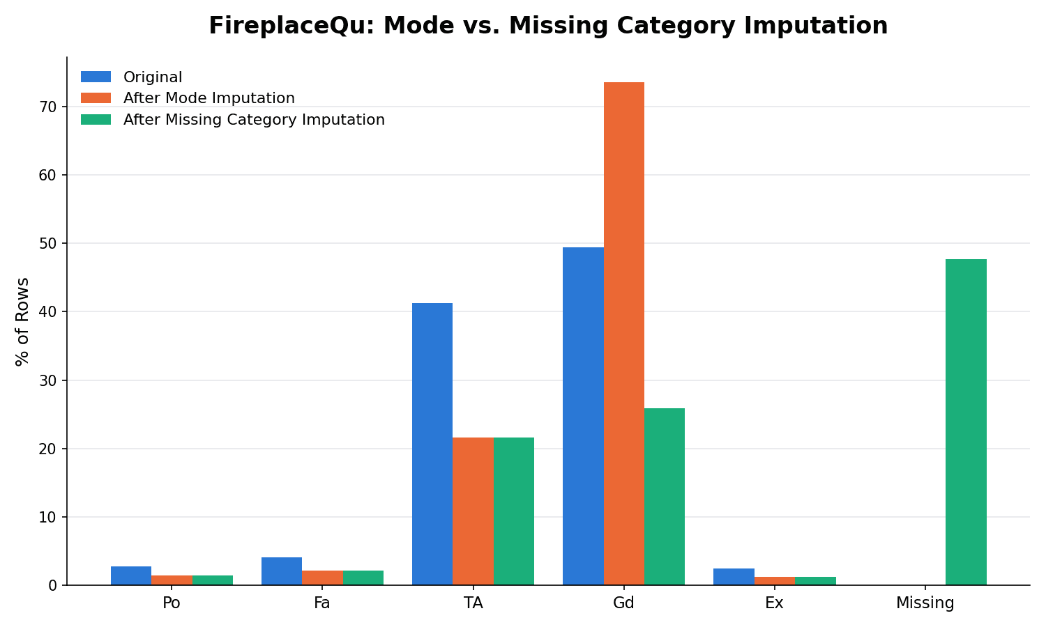
The difference from mode imputation is visible immediately: Gd and TA don't get warped, they shrink proportionally as "Missing" claims its own honest 47.69% slice, but their ratio to each other stays intact, Gd was 1.20x TA originally (49.43 / 41.24) and stays almost exactly 1.20x after (25.86 / 21.58). Mode imputation broke that relationship; missing category imputation preserves it.
With scikit-learn, this is SimpleImputer with a constant strategy, same as arbitrary value imputation was for numerical columns:
si = SimpleImputer(strategy='constant', fill_value='Missing')
si.fit_transform(X_train[['FireplaceQu']])
Summary Cheat Sheet
| Technique | scikit-learn | Use When |
|---|---|---|
| Most Frequent (Mode) | SimpleImputer(strategy='most_frequent') | MCAR, light missingness, one category clearly dominates |
| Missing Category | SimpleImputer(strategy='constant', fill_value='Missing') | not MCAR, heavy missingness, no dominant category |
What's Next?
This post covered the two go-to techniques for filling in categorical gaps: mode imputation, which works cleanly only when one category already dominates, and missing category imputation, which sidesteps the guessing problem entirely by giving unknown values their own honest label. Both are univariate: each column gets filled using only its own data. The next posts in this series cover Random Sample Imputation, which applies to numerical and categorical columns alike, and multivariate imputation (KNN Imputer, Iterative Imputer), which fills gaps using the other columns instead of just the column's own statistics.