Ch.68: Agglomerative Hierarchical Clustering

Inspired by: YouTube

The K-means post ended with a working algorithm: pick $K$, place random centroids, repeat assign-then-move until nothing changes. That algorithm has a real weakness worth seeing directly before reaching for its replacement.

1. Where K-Means Actually Fails

K-means clusters by distance to a centroid, which quietly bakes in an assumption: clusters are roughly round blobs. Hand it a few other shapes and that assumption breaks:

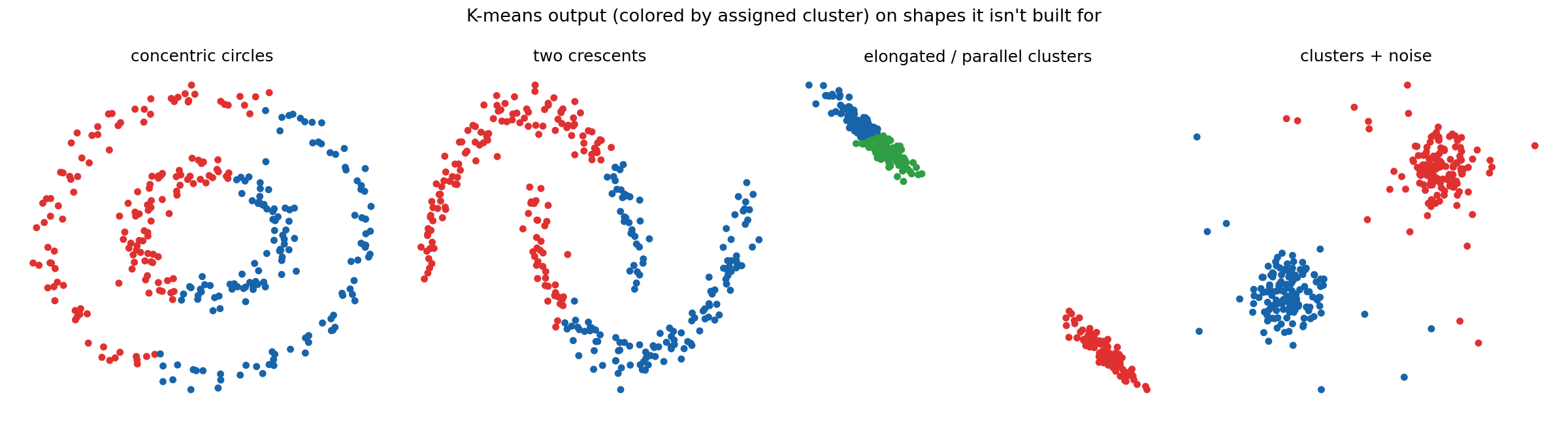
In every panel, K-means does exactly what it's built to do, minimize distance to a centroid, and in every panel that's the wrong objective for the actual shape of the data. Concentric circles need to be split by ring, not by a line through the middle. The crescents need to be split by moon. The elongated cluster is one group that happens to be stretched, not two groups cut across the middle. And K-means has no concept of "this point doesn't belong to any cluster," so stray noise gets forced in wherever it's nearest.

K-means works best specifically on spherical (or hyperspherical, in higher dimensions) clusters. Two other families of algorithms exist to handle the cases it doesn't: density-based clustering (DBSCAN, covered separately) and hierarchical clustering, the subject of this post.

2. Agglomerative vs Divisive

Hierarchical clustering comes in two directions. Agglomerative clustering works bottom-up: start by treating every single point as its own cluster, then repeatedly merge the two closest clusters until only one remains. Divisive clustering works top-down: start with all points in one cluster, then repeatedly split the least cohesive cluster until every point is alone.

Agglomerative is the one actually used in practice, for a fairly simple reason: deciding which two clusters are closest and merging them is a much better-defined operation than deciding how to best split a cluster into two. The rest of this post covers agglomerative clustering specifically.

3. The Core Idea: Merge the Closest Pair, Repeat

Six points, clustered by hand, to build the intuition before any code:

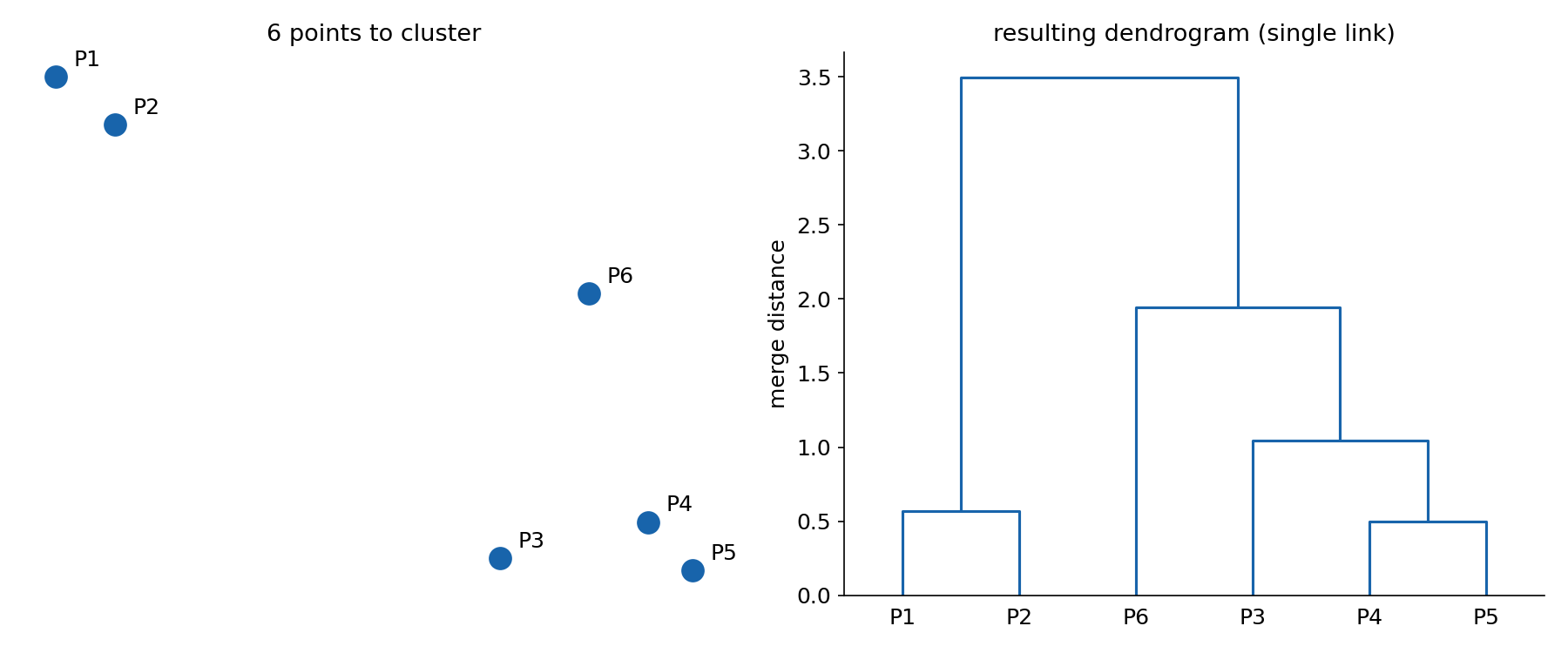
Every point starts as its own cluster, six clusters for six points. The two closest points, P4 and P5, merge first. Separately, P1 and P2 are also close, so they merge too. Now there's a cluster of ; P3 turns out to be closer to that cluster than to anything else, so it joins, forming . P6 is next closest to that group, so it joins too. Finally, the only two clusters left, and , merge into one.

Every merge gets recorded, and that record, drawn as a tree, is called a dendrogram. The height at which two clusters merge represents how far apart they were when they merged. Reading the dendrogram back tells the full merge history: P4-P5 were the closest pair overall, P1-P2 merged independently and later than P4-P5, and the last, highest merge (combining the two main branches) was the least natural one, forced only because the algorithm runs until a single cluster remains.

4. The Algorithm, as Pseudocode

Stated generally, for $n$ points:

1. Build a proximity matrix: an $n \times n$ table where entry $(i, j)$ is the distance between point $i$ and point $j$. The diagonal is all zeros, since every point's distance to itself is zero.
2. Treat every point as its own cluster.
3. Loop: find the two closest clusters in the current proximity matrix, merge them into one, and update the matrix, removing the two merged rows/columns and adding one new row/column for the merged cluster.
4. Stop once only one cluster remains.

Step 3's update is where this gets genuinely tricky. The distance between two points is unambiguous, Euclidean distance between two coordinates. The distance between two clusters, each potentially containing many points, is not: "how far apart are these two groups?" has more than one reasonable answer, and the different answers are exactly what separate the different types of agglomerative clustering.

5. Four Ways to Measure Inter-Cluster Distance

Given two clusters, each with potentially many points, scikit-learn's AgglomerativeClustering supports four strategies (the linkage parameter) for turning all the pairwise point-to-point distances between the two clusters into a single number:

• Single link (linkage="single"): the distance between the two closest points, one from each cluster. Cheap to reason about, and it makes well-separated clusters trivial to find correctly. Its failure mode is chaining: a thin trail of points bridging two otherwise-separate blobs gets treated as evidence that the blobs are close, merging them into one.
• Complete link (linkage="complete"): the distance between the two farthest points, one from each cluster, the opposite extreme. This resists chaining, since a single close pair of points isn't enough to trigger a merge, the farthest pair still has to be close too. Its failure mode is the opposite kind of distortion: a genuinely large cluster can get split apart, because its farthest internal points make it look less cohesive than it actually is.
• Average link (linkage="average"): average every pairwise distance between the two clusters' points. A compromise between single and complete, inheriting a milder version of each one's behavior rather than either extreme.
• Ward's method (linkage="ward", scikit-learn's default): merge whichever pair of clusters produces the smallest increase in total within-cluster variance. Concretely, for two candidate clusters, compute their combined centroid, sum the squared distances from every point in both clusters to that shared centroid, then subtract out the variance that was already present inside each cluster separately, what's left is the "cost" of merging them. Like average link, it sits between single and complete in practice.

Written out, Ward's merge cost for two clusters $A$ and $B$, with centroids $\mu_A$ and $\mu_B$, and $\mu_{A \cup B}$ the centroid of all their points combined, is exactly that three-part recipe:

The first term is the spread of the merged cluster around its shared centroid; the other two are the spread each cluster already had on its own. With a little algebra, the whole expression collapses into a form that only needs the two centroids and the two cluster sizes $n_A$ and $n_B$:

This second form shows what Ward actually rewards. The $\lVert \mu_A - \mu_B \rVert^2$ part says clusters whose centers are close are cheap to merge, like any other linkage. The $\frac{n_A n_B}{n_A + n_B}$ weight is the new part: it grows with cluster size, so two big clusters cost more to merge than two small ones at the same centroid distance. That pushes Ward toward absorbing small clusters first and producing clusters of similar size. One detail if you read the dendrogram's merge heights: SciPy's linkage(..., method="ward") reports $\sqrt{2\,\Delta(A, B)}$ as the height rather than $\Delta(A, B)$ itself. Since that's a monotonic rescaling, the merge order and the shape of the tree are unchanged; only the numbers on the vertical axis differ.

The same two clusters, with each method's defining computation drawn directly on top of the points:

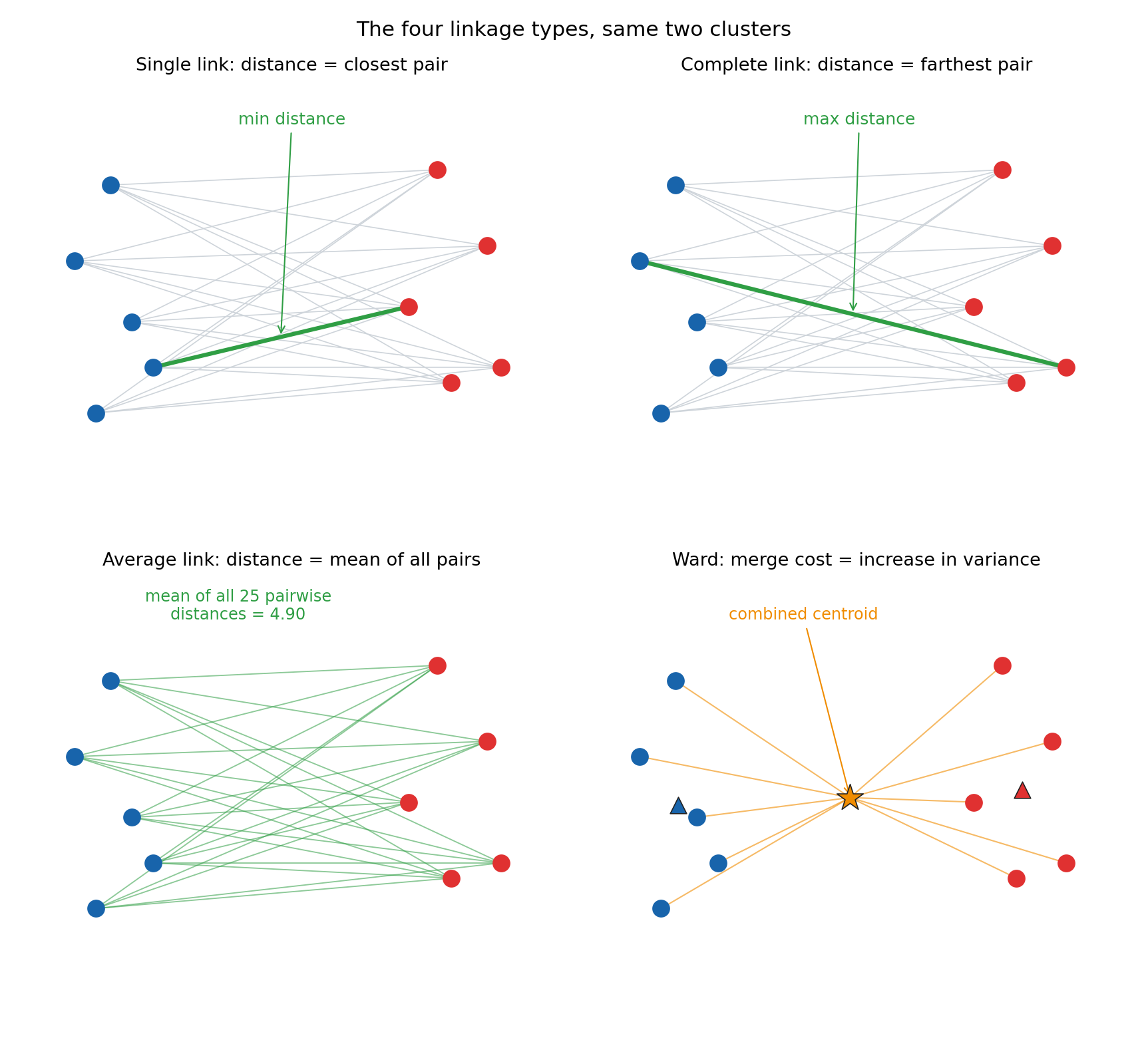
Single and complete link both reduce the entire relationship between two clusters down to one specific pair of points, just different pairs (the nearest and the farthest, respectively), while discarding every other distance in the panel's faint background mesh. Average link keeps all of them, just flattened into a single mean. Ward works differently again: instead of picking or averaging point-to-point distances at all, it asks how far every point in both clusters sits from their one shared (combined) centroid, which is a direct stand-in for how spread out the merged cluster would become.

The chaining failure mode is worth seeing directly, since it's single link's defining weakness. Two well-separated blobs connected by a thin, dense trail of bridge points:

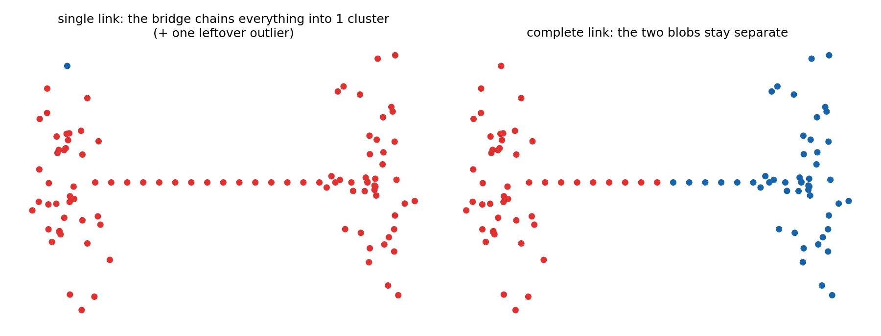
Single link, asked for 2 clusters, produces one giant cluster covering almost everything plus a single leftover point, exactly the chaining failure: each bridge point is close to its neighbor, so the merge chain never has a reason to stop at the gap between the two blobs. Complete link, run on the identical data with the identical request for 2 clusters, recovers the two blobs cleanly, because a bridge point being close to one blob doesn't make the two blobs' farthest points close to each other.

None of the four linkage types is simply "better," they fail in different ways on different data, which is itself the point: hierarchical clustering's flexibility comes from choosing among them, not from one universally correct default (even though Ward is scikit-learn's default and a reasonable starting point).

6. Choosing the Number of Clusters from the Dendrogram

Agglomerative clustering, run to completion, always ends at exactly one cluster, so "how many clusters are there" isn't answered by the algorithm itself any more than it was for K-means. The dendrogram makes the answer readable directly: find the tallest vertical line that no horizontal line crosses, and cut through it.

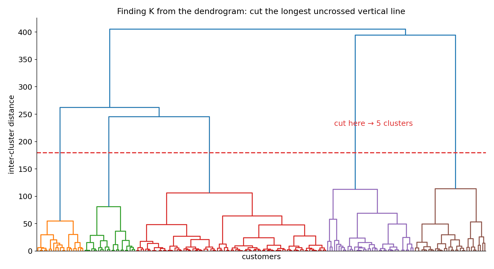
The cut line sits in the largest unobstructed vertical gap, the four highest merges in this dendrogram happen at heights roughly 406, 395, 263, and 246, then the next merge drops all the way down to about 114, a large jump. Cutting anywhere in that gap crosses exactly 5 of the tree's branches, so 5 is the natural number of clusters this dendrogram is suggesting. The vertical distance at any merge point is exactly the inter-cluster distance from Section 5, the same quantity single link, complete link, average link, or Ward's method was computing all along.

7. Full Example: Segmenting Mall Customers

The classic dataset for this algorithm is a 200-row mall customer dataset ([CustomerID, Genre, Age, Annual Income, Spending Score]), using only the last two columns:

import pandas as pd
import scipy.cluster.hierarchy as shc
from sklearn.cluster import AgglomerativeClustering
 
customer_data = pd.read_csv("shopping_data.csv")
data = customer_data.iloc[:, 3:5].values  # Annual Income, Spending Score
 
dend = shc.dendrogram(shc.linkage(data, method="ward"))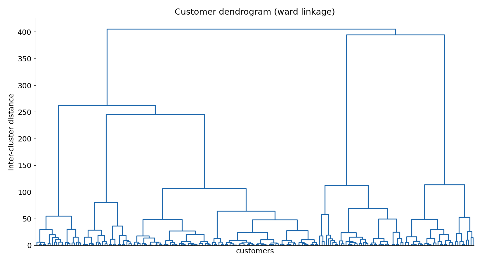

Applying the cut rule from Section 6 to this exact dendrogram gives $K=5$:

cluster = AgglomerativeClustering(n_clusters=5, metric="euclidean", linkage="ward")
labels = cluster.fit_predict(data)

(Older scikit-learn versions name this parameter affinity instead of metric; both set the point-to-point distance measure, with euclidean as the default.)

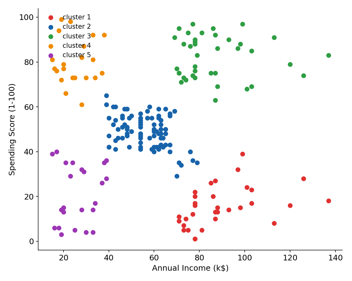
Five groups fall out cleanly: customers with low income but high spending, low income and low spending, mid income and mid spending clustered densely in the center, high income with high spending, and high income with low spending, a genuinely useful segmentation for a marketing team deciding who to target with which offer, with no manual boundary-drawing required.

A natural follow-up exercise: run the same recipe on a countries-of-the-world dataset (GDP, population, surface area, and similar columns), and see which countries end up closest to any one country of interest in the resulting dendrogram. That exercise doesn't have a companion notebook here, there's no dataset-specific trick involved beyond everything covered above, just a different CSV through the same shc.linkage and AgglomerativeClustering calls.

8. Benefits and the One Big Limitation

Two genuine advantages over K-means: hierarchical clustering handles a much wider variety of cluster shapes (choosing single, complete, average, or Ward linkage to suit the data, rather than being locked into one geometric assumption), and the dendrogram itself is a reusable artifact, it records, for every point, exactly which other points it's closest to and in what order, information a K-means run simply doesn't produce.

The cost is memory. The proximity matrix is $n \times n$, every point's distance to every other point, and that grows quadratically with no way around it. For $n = 10^6$ points, the matrix needs on the order of $10^{12}$ entries; stored as 8-byte floating point numbers, that's roughly $8 \times 10^{12}$ bytes, on the order of several terabytes, in RAM, for the distances alone. Past a dataset of a few tens of thousands of rows, this algorithm simply stops being usable, which is the real reason it isn't the default choice for large-scale clustering the way K-means or DBSCAN are.

9. What to Take Away

• K-means' weakness is structural: it measures distance to a centroid, which only matches data that's actually shaped like round blobs. Concentric circles, crescents, elongated clusters, and noisy data all break that assumption.
• Agglomerative clustering starts with every point as its own cluster and repeatedly merges the two closest clusters until one remains, recording the full merge history as a dendrogram. Divisive clustering runs the opposite direction but is rarely used, since splitting is a harder-defined operation than merging.
• The real design decision is linkage, how "distance between two clusters" gets defined: single link (closest pair, prone to chaining), complete link (farthest pair, prone to splitting large clusters), average link (mean of all pairwise distances), and Ward's method (minimum increase in within-cluster variance, scikit-learn's default).
• The number of clusters is read off the dendrogram directly: cut through the tallest vertical line that no horizontal line crosses, and the number of branches crossed is the suggested $K$.
• The proximity matrix's $O(n^2)$ memory requirement is the algorithm's binding constraint, it becomes impractical well before K-means or DBSCAN would, on the same hardware.